Optimization Step
The Optimization section contains the following tabs:
Optimize Tab
The Optimize tab contains the following elements:
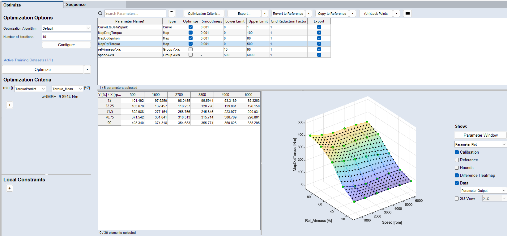
Optimization Options
The options are saved per optimizer. They are retained when you switch between optimizers.
Optimization Algorithm
Select the algorithm or sequence you want to use for optimization. For an explanation of the algorithms, see Optimization Algorithms.
Enter the maximum number of iterations to be performed during optimization.
If the optimizer converges before reaching the total number of iterations, it will stop earlier.
 Configure
To customize the optimizer settings, click Configure. For an explanation of the options, see Optimizer Options.
Active
Displays the number of active datasets out of the total number of datasets.
Click to open the Active Datasets window where you can select which datasets to activate.
Starts the optimization.
The  button opens a context menu where you can choose between:
-
Optimize
-
Export Job to M Script: Exports the optimization information as MATLAB® script file (*.m). Use the script file to perform the optimization in another instance of ASCMO-MOCA, such as on another device.
-
Export Job to Docker: Exports the optimization information as *.docker.moca file. Use the file to perform the optimization in a Docker container, e.g., in the cloud.
Optimization Criteria
Criterion row
The criterion to be minimized. The first drop-down lists all function nodes and Remove Remove deletes the optimization criterion. The second drop-down lists the imported data channels, function nodes created in the Function Step, Remove, and 0. You can create a constant as a criterion by selecting <Select Contstant>.
The optimizer will then attempt to find a set of parameter values that minimizes the quadratic deviation of the two selected quantities.
0 means that the model prediction is minimized. You can use this to determine more complicated optimization formulas: create a function node with your optimization formula, then minimize that node.
Instead of the quadratic deviation (Yprediction-Ytraining).^2, you want to minimize (Yprediction-Ytraining).^4. Do the following:
-
Create a function node myLastNode = (Yprediction-Ytraining).^2.
-
Specify the optimization criterion min(MyLastNode-0)^2.
With that, min(Yprediction-Ytraining)^4 is computed during optimization.
RMSE
The current RMSE (see Variables RMSE and R2) of the optimization criterion.
 Add a new Optimization criterion
Adds a new criterion row.
Local Constraints
Constraint row
-
first drop-down
The channel or function node to be limited. Available selections are all imported data channels and function nodes. You can create a constant by selecting <Select Contstant> to define a constraint like output < constant for example.
-
second drop-down
The comparison operators. Available selections are <=, = and >=.
-
third drop-down
The channel or function node to be used as limit. Available selections are all imported data channels and function nodes. You can create a constant by selecting <Select Contstant> to define a constraint like output < constant for example.
-
 Remove this constraint
Violation
Shows the sum of constraint violations.
Add a new Optimization constraint
Adds a new constraint row.
Parameter
Optimization Criteria
Opens the "Parameter Optimization Properties" window. See Setting Optimization Criteria for a Parameter for details.
Export
Click Export to open the Export Parameters window, where you can specify the location, name, and file type for the parameters to be exported.
To select only certain parameters for export, use the checkboxes in the Export column of the Parameters table.
The button opens a  drop-down menu.
|
Parameters (default) |
Opens an open file dialog, where you can specify the location, name, and file type for the parameters to be exported. |
|
Bounds |
Exports the bounds of map, curve and cube-3D/cube-4D parameters to a file. |
|
Parameters and Bounds |
Exports all parameters, their values and bounds (only map, curve and cube-3D/cube-4D parameters) to a file. |
|
Patch Parameter or Variant in Existing DCM File |
Exports the selected parameters or variants and patches them into an existing DCM file. This way only the changed parameters can be exported and added to the existing file. |
|
Selected Parameters to Bosch iLrn (offline) |
Exports the selected parameters, curves, maps and cubes as BIN and DCM file as iLrn (offline) flatbuffer for Bosch ECUs. |
|
Compressed Model to M-script |
Exports parameters of type Compressed Model to an M script file so that the model can be executed in MATLAB®. |
|
Compressed Model to Bosch AMU |
Exports parameters of type Compressed Model to a DCM/CDFX file for Bosch AMU. |
|
Parameter list as LAB |
Exports parameter names to a LAB file for easy selection in ETAS INCA. |
|
Note |
|---|
|
Available export formats are DCM Files (*.dcm), several comma-separated value formats (*.csv), several Excel formats (*.xls, *.xlsx,*.xlsm), calibration data files (*.cdfx), M-scripts (*.m), and LAB files (*.lab). |
See also Exporting Parameters and/or Bounds.
Revert to Reference
Click Revert to Reference to reset the optimized parameter values to the reference values (original).
The  button opens a drop-down menu.
Copy to Reference
Click Copy to Reference to copy the current values of the parameter set to the reference parameter set (see Parameters Step). The values of the reference parameter set are overwritten.
The button opens a drop-down menu.
(Un)Lock Points
Click Lock Points to exclude the selected grid points from optimization.
The button opens a drop-down menu.
|
Note |
|---|
|
Single grid points with or without data can be locked or unlocked via context menu (right-click). |
 Menu button
Opens a drop-down menu.
Parameters table
Lists all parameters in the project.
Use F2 or Double-click a cell to edit the value.
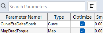
Use the search bar to search for a parameter name. Use  to clear the search.
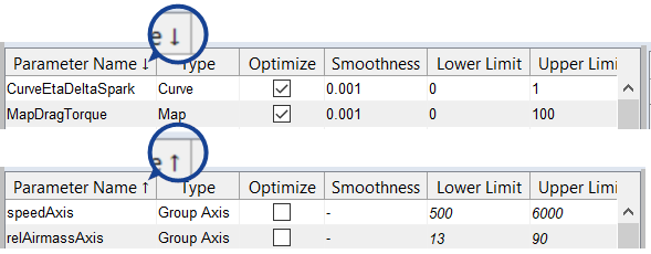
The table can be sorted in ascending or descending order using the table header. Clicking the table header will sort the table by the corresponding column.
You can use the standard Ctrl/Shift selection functions in the table
Right-click in the table to open the context menu of the selected parameters.
In addition to the parameter names and types, the table contains the following columns.
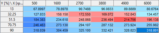
Shows the values of the selected parameter. For curves/maps/cubes, the axes are displayed as the column/row headers of the table. The first axis (x) is displayed as the column header. The second axis (y) is displayed as the row header. The cells display the parameter values.
The appearance of the table depends on the parameter type. For 3D and 4D cube parameters, the third and fourth axes are displayed as separate lists. For parameters of compressed model types, the inputs are displayed in a separate list.
Use F2 or Double-click a cell to edit the value.
You can use the standard Ctrl/Shift selection functions in the table
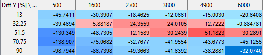
Differences between the reference and working parametersets are visually distinguished in the table using different shades of red and blue. Cells appear redder when the reference value is lower and bluer when it is higher, with the darkness of the color reflecting the extent of the difference.
Use the Difference Heatmap checkbox in the Show area to activate/deactivate the color coding.
When the Reference option of the Show area is activated, the table shows the differences between the reference and working parametersets.
To open the context menu of the selected parameter value, right-click in the selection.
Shows a plot of the parameter selected in the parameters table.
For scalars, curves, maps, and cubes, the plot area contains the following elements:
Parameter Window
|
Note |
|---|
|
Only available for curve and map parameters. |
Opens the Parameter window, where you can edit the bounds.
Show
Select whether a parameter plot or a heatmap should be displayed.
The following options are only available for parameter plots:
Activate the corresponding checkbox to show:
- the parameter from the working parameterset (Calibration)
-
the reference/initial parameterset (Reference, see also Dealing with Reference Parameters)
-
When activated, the Parameter value table shows the differences between the reference and working parameter.
-
-
the upper and lower bounds (Bounds, only available for curve and map parameters)
-
the color-coded differences in the parameter value table (Difference Heatmap)
-
the data points as black dots in the plot. Select the data to display from the drop-down list (Data).
The signals of the project and a special signal Parameter Output are available. Parameter Output shows the input signals evaluated by the parameter. This is useful to see the distribution of the input signals.
2D View
Activate the checkbox to display the parameter plot as a 2D plot. Use the drop-down menu to select whether to display the X-Z or the Y-Z axes as the X and Y axes of the 2D plot.
The third axis data can be displayed as connected points in the 2D plot. Therefore select the corresponding row or column in the parameter value table above. Select multiple values (Ctrl or Shift)in the table to display multiple values in the plot.
Sequence Tab
The Sequence tab contains the following elements:
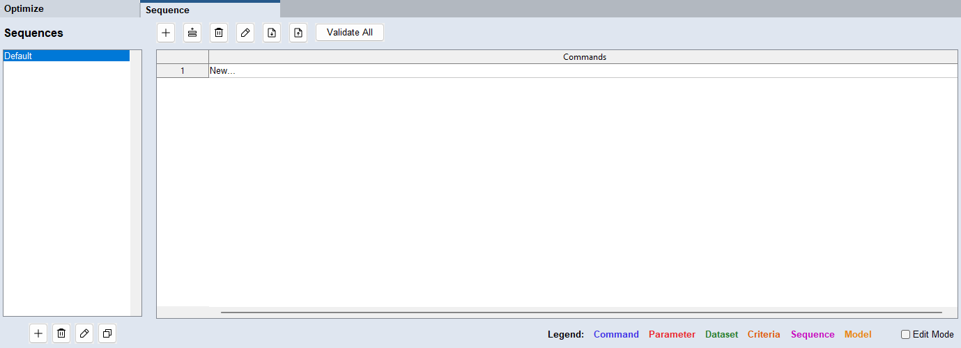
Sequences
Lists all defined sequences. To edit the sequence, use the buttons below the list:
 Add a new sequence to the list.
 Delete the selected sequence.
 Rename the selected sequence.
 Duplicate the selected sequence.
Commands
Lists all commands contained in the sequence.
You can use the standard Ctrl/Shift selection functions in the table
To edit the commands, use the buttons above the list:
Add a new command to the end of the sequence via the Add/Edit Command window.
 Insert a command above a selected command via the Edit/Add Command window.
Delete the selected commands from the sequence.
Edit the selected command.
 Import a MOCA sequence (*.mocaseq). It is a human-readable file that you can edit and then re-import using the Import button.
 Export the selected sequence (*.mocaseq).
 Validate all commands in the list.
For a list of all commands, see Add/Edit Command.
See also
Step 6: Optimization (tutorial)