Optimization Algorithms
In the Optimization step, you can choose from the following optimization algorithms:
Gradient descent optimization starts with the working parameter set as initial values and uses the gradient of the cost function to iteratively follow the direction of the steepest descent to the minimum of the cost function. The gradient descent optimizer only finds a local minimum, so the starting position of the optimization is important.
ASCMO-MOCA calculates the gradients of the function analytically. Gradients from external models, such as Simulink or FMU models, are computed using the finite difference method. This allows the optimizer to find the local minimum quickly and with a minimum number of function evaluations. The memory consumption is at least the number of data points multiplied by the number of parameters and multiplied by two for the optimization algorithm itself.
Global optimizers are gradient-free optimizers that try to find a global optimum. They start with several random candidate solutions to the optimization problem spread over the entire search space. Then the search space is iteratively narrowed down to good, more accurate solutions. The optimization may not hit the optimum perfectly, so you can start with a global optimization to find the global optimum, and then continue with a gradient descent optimization to refine the result.
A typical optimization problem in ASCMO-MOCA is the optimization of maps and curves. Such an optimization problem usually has many parameters (e.g., a 20x20 map has 400 parameters), and a global optimizer may require many iterations to find a good solution.
Being gradient-free, global optimization can find a solution when the gradients of a function/model are not continuous. This happens when your model is implemented with a fixed-point representation of numbers or parameters and inputs or outputs are discrete. It can also happen if your model is implemented with 32-bit instead of 64-bit floating point numbers.
Default (Gradient Descent)
This is a gradient descent least squares optimizer. It was chosen as the default optimizer because it performs well when the optimization task has many parameters, which is likely when using maps and curves.
The residuals enter the optimization algorithm as a vector, so the optimizer gets 100 residuals for a dataset with 100 data points. This is computationally expensive, but leads to good optimization results.
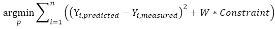
The residuals are implicitly squared by the optimizer, so the difference from a reference value is always minimized. To do a minimization or maximization, you must explicitly provide a low/high value to optimize against.
The output is in the range 0 to 1000. To do a maximization, define the optimization criterion as minarg(y(x)-1000).
Local constraints enter the optimization as part of the sum formula (W * Constraint). In the context of ASCMO, this is called a soft constraint. The weight of such a local constraint is increased every 10 iterations until the constraint is satisfied.
During optimization, the weight of the constraint is increased if the constraint is violated. This may not be sufficient, and the constraint may still be violated after optimization.
When to use: The Gradient Descent Optimization is ideal for the typical problems MOCA addresses. It is fast and delivers good results, though it requires substantial memory. Other optimization algorithms should be considered only in specific situations outlined below.
Usage: Gradient descent optimization is ideal for the typical problems that MOCA addresses. It is fast and gives good results, although it requires a lot of memory. Other optimization algorithms should be considered only in the specific situations described below.
Respect Constraints (Gradient Descent)
This is also a gradient descent least squares optimizer, but it takes constraints into account.
The constraints are treated by the optimizer as hard bounds. The default optimizer should be preferred unless the constraints are violated. Use this algorithm if a constraint is violated after optimizing with the default optimizer.
Usage: This optimization algorithm is useful when local constraints are violated after running an optimization. It's recommended to first try the default optimizer and increase the weight of the local constraints (e.g. 10, 100, 1000, etc.). If this approach fails, this algorithm may find a solution within the constraints.
Gradient-free Optimizer
The gradient-free Optimizer uses a simplex algorithm for optimization. The algorithm does not depend on gradients and therefore requires more iterations than a gradient descent algorithm. The solutions are typically not as good as those of a gradient descent optimizer.
Use this gradient-free optimizer when the gradients of the function/model are not continuous. This happens when your model is implemented with a fixed-point representation of numbers or parameters and signals are discrete. It can also happen if your model is implemented with 32-bit instead of 64-bit floating point numbers.
Usage: This optimization algorithm is suitable for external models that are insensitive to small parameter changes, such as those that use fixed-point representation internally. If an external model uses single precision (32-bit) instead of double precision, consider increasing the finite difference factor to 20,000 and using the default optimizer.
Surrogate Optimizer (Global Optimization)
The Surrogate Optimizer tries to find a global optimum. It first builds a surrogate model and then optimizes it instead of the original function/model. This can be useful if the function/model evaluation takes a long time.
Usage: This optimization algorithm is useful when evaluating an external model is time-consuming. A surrogate model, which is evaluated quickly, is built for optimization purposes.
Genetic Algorithm (Global Optimization)
The Genetic Algorithm tries to find a global optimum. It is inspired by natural selection and the exchange of genomes. It starts with random candidate solutions, here called a population, see Wikipedia: Genetic Algorithm for more details. The size of the population strongly influences the memory consumption. An optimization task with many signals and/or data can lead to out-of-memory problems. Reducing the population size frees up memory. The algorithm performs a vectorization with all candidate solutions and can perform model evaluations of FMU and TSim models in parallel.
Usage: This optimization algorithm is a gradient-free optimization algorithm suitable for insensitive models. Its primary purpose is to find a global minimum, especially when the default optimizer may get stuck in a local minimum. The algorithm uses less memory than the default optimizer, but may take longer to achieve similar results.
Simulated Annealing (Global Optimization)
Simulated Annealing tries to find a global optimum. It starts with random candidate solutions at the beginning of the optimization. Due to a high initial temperature, large parameter changes are possible. Over several iterations, the temperature decreases, limiting possible parameter changes and allowing more accurate solutions to be found. See Wikipedia: Simulated Annealing for more details. The number of particles strongly affects the memory consumption. An optimization task with many signals and/or data can lead to out-of-memory problems. Reducing the number of particles frees up memory.
Usage: This optimization algorithm is a gradient-free optimization algorithm suitable for insensitive models. Its primary purpose is to find a global minimum, especially when the default optimizer may get stuck in a local minimum. The algorithm uses less memory than the default optimizer, but may take longer to achieve similar results.
Particle Swarm (Global Optimization)
Particle Swarm tries to find a global optimum. It starts with random candidate solutions, called particles. The particles have a position and a velocity. It starts with a high velocity and over several iterations the velocity decreases, allowing more accurate solutions to be found, see Wikipedia: Particle Swarm Optimization for more information. An optimization task with many signals and/or data can lead to out-of-memory problems. Reducing the number of particles frees up memory. The algorithm performs a vectorization with all candidate solutions and can perform model evaluations of FMU and TSim models in parallel.
Usage: This optimization algorithm is a gradient-free optimization algorithm suitable for insensitive models. Its primary purpose is to find a global minimum, especially when the default optimizer may get stuck in a local minimum. The algorithm uses less memory than the default optimizer, but may take longer to achieve similar results.