Driving Cycle Manager
Calibration menu > Driving Cycles
Driving cycles are produced by different countries and organizations to assess the performance of vehicles in various ways, as for example fuel consumption and polluting emissions. Another use for driving cycles is in vehicle simulations. More specifically, they are used in propulsion system simulations to predict performance of internal combustion engines, transmissions, electric drive systems, batteries, fuel cell systems, and similar components. The driving cycles of the project can be managed in the Driving Cycle Manager window.
The Driving Cycle Manager window contains the following elements:
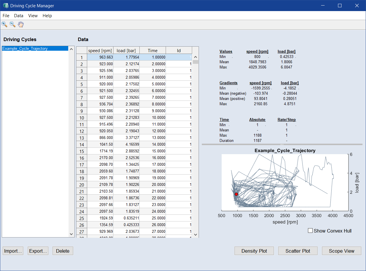
Driving Cycles list
On the left side there is a list of the driving cycles currently available in the project. One or more driving cycles can be selected.
-
 Import: Opens a file selection window for importing a driving cycle. Cycle data in the following formats can be imported: Excel (*.xls, *.xlsx, *.xlsm), MDA export (*.ascii), comma-separated values (*.csv, *.txt), MDF (*.dat, *.mf4, *.mdf, *.mdf3).
 -
Export: Exports the currently selected driving cycles to an Excel file (*.xls, *.xlsx), or comma-separated values (*.csv).
-
Delete: Deletes the currently selected driving cycles from the project.
Data table
The Data table in the middle part shows the selected driving cycles as data table. The following columns are available:
- <first OP axis>
- "<second OP axis>"
- "Time"
- ID (only available if 2 or more lists are selected)
- "<third OP axis>" (only available if one list with 3 or 4 operating point axes is selected)
- "<fourth OP axis>" (only available if one list with 4 operating point axes is selected)
If you select a row in the data table representing a cycle, the respective point is shown as red dot in the plot on the right side. If desired, you can select several rows. In that case, the trace of those points is  marked by a red line and the statistics part is updated by just considering the selected points.
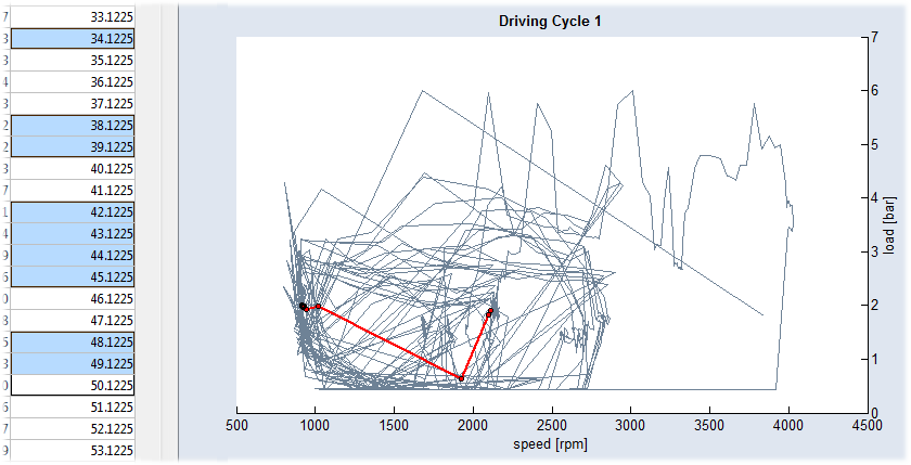
The driving cycles can be edited by changing or deleting rows in the table. Note that the edit mode is deactivated if you selected more than one driving cycle in the list on the left side. It is possible to select a point by clicking it in the plot.
Statistics area
On the right side, there are some statistical evaluations of the driving cycles, as well as a plot of the cycles.
If you activate the Show Convex Hull checkbox, the convex hull of the selected cycles is plotted.
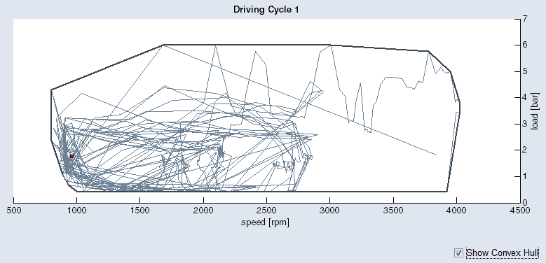
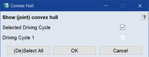
You can determine which driving cycles are used for the calculation of the convex hull in the Convex Hull window opened with View > Convex Hull Selection.
Opens a density plot window for each currently selected driving cycle. If a driving cycle contains three or four operating point axes, the window contains two density plots.
The trajectory of the driving cycle is colored, and the colors represent the probability of presence in the speed / load range. See also Density Plot <driving cycle> Window.
Opens a scatter plot of the currently selected driving cycles, showing the points of the respective cycles as well as the gradients. By holding the left mouse button, rectangles can be drawn and points inside the rectangle can be deleted. See also Driving Cycles Scatter Plot and Driving Cycles Time .
Opens a scope view for each currently selected driving cycle, showing a plot of the inputs over the time. See also Scope View <driving cycle> Window.
See also
Using a Driving Cycle to Assign OP Weights