Multi-Criteria Optimization
Optimization tasks frequently lead to the situation that the reduction, e.g. of an emission variable, is associated with the increase of other values, such as consumption. The multi-criteria optimization is available for the optimization of such "opposite" outputs.
Change settings of the multi-criteria optimization
-
Select Optimization > Multi Result.
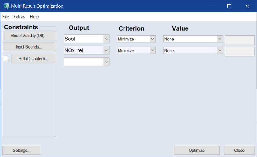
The Multi Result Optimization window opens.
-
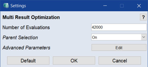
In the Multi Result Optimization window, click Settings.
Note
The Edit button to customize the advanced parameters is only available if the Advanced Settings are enabled (see Enable/Disable Advanced Settings ).
-
In the Number of Evaluations field, specify the maximum number of function evaluations across all generations.
The number of evaluations should be approximately 200 times the number of children-generating parents (Parent Population Size in the advanced parameters).
-
In the Parent Selection field, activate (On) or deactivate (Off) involvement of the parents in evaluation and recombinations of new generations.
For more information, see Evolutionary Algorithm (Parent Selection vs. Survivor Selection) .
- Click OK to confirm the settings.
Restrict the range of parameter variation (Constraints)
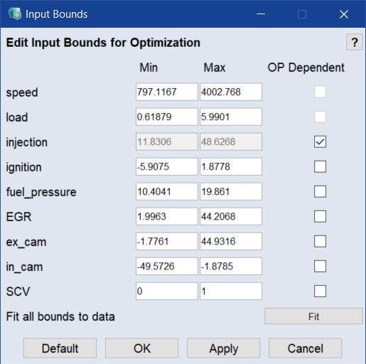
For every input, the range to be considered for the modeling can be defined here. To do so, proceed as follows:
-
In the Multi Result Optimization window, click Input Bounds.
-
In the Input Bounds window, click Fit to fit all bounds to measured data.
Or
Do one of the following for each input you want to limit:
- Enter the range of valid parameter variation (Min/Max) for optimization.
-
Activate the OP Dependent checkbox.
The Map Bounds window opens for the respective input. Here you can manually specify the range of parameter variation using the defined grid points.
-
Click OK to apply your settings and close the Input Bounds window.
Note
For more information regarding the definition of valid parameter variation using OP-dependent input bounds, see Calibration .
Limiting the optimization results
You can limit the optimization results to the range of valid model output in different ways.
-
In the Multi Result Optimization window, activate the option next to the Hulls button.
This limits the range of parameter variation to the data within the specified hull (In/Outputs > Hull on Inputs).
-
Click Model Validity.
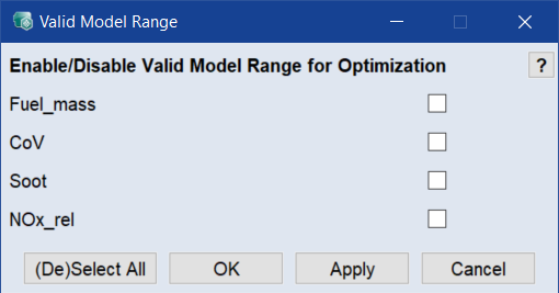
- In that window, activate each element you want to limit to the valid model range.
-
Click OK to apply your settings and close the Valid Model Range window.
Note
The options in the Valid Model Range window should always be enabled so that the solutions found by the optimizer can also be set later. A prerequisite for the use of this option is that the corresponding variables have a meaningful validity range. If not, it would be an indication for a faulty model training.
Multi-criteria optimization
- If necessary, open the Multi Result Optimization window.
- Remove the outputs Fuel_mass and CoV by selecting Remove in the Output column.
-
Select the Minimize optimization criterion for the two outputs Soot and NOx_rel.
- Open the operating points manager (cf. Operating points manager (A: input fields for operating point values, B: operating points, C: measurement points, D: convex hull of the plot)).
-
In that window, select an operating point at which you want to perform the optimization, e.g.,
- 2000 rpm
- 2 bar mean effective pressure
- Lock speed and load as described in Defining the operating point.
-
In the Multi Result Optimization window, click Optimize.
The optimization starts The progress is displayed in the status bar at the bottom edge of the window.
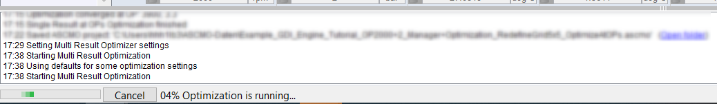
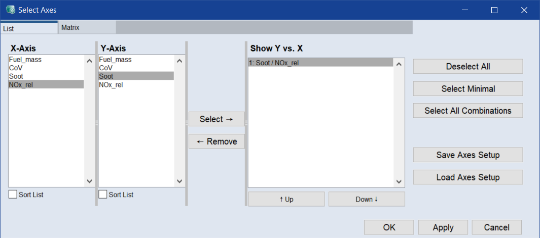
Upon completion, the Select Axes window opens.
-
In that window, in the List tab or in the Matrix tab, select the pair of axes to be displayed.
-
In the List tab, select NOx_rel as X axis and Soot as Y axis, then click Select →.
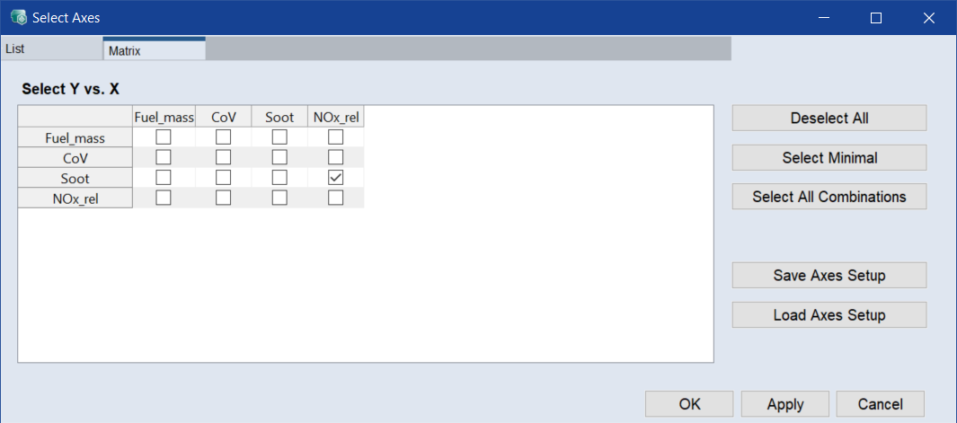
-
In the Matrix tab, activate the checkbox in the Soot row, NOx_rel column.
-
-
Click OK.
-
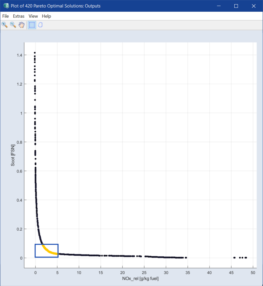
The plot for the mutual dependency between soot and nitrogen oxide emission is displayed.
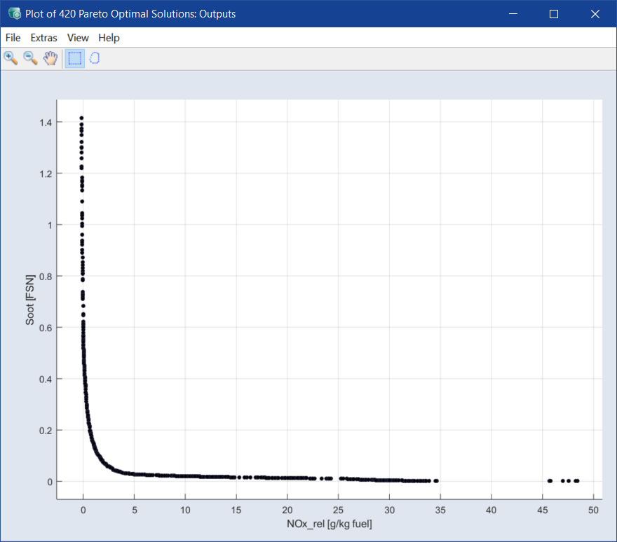
Note
All points on this curve are Pareto-optimal solutions with respect to the optimization criteria.
In addition, a second window opens in which dependencies between inputs and outputs can also be displayed.
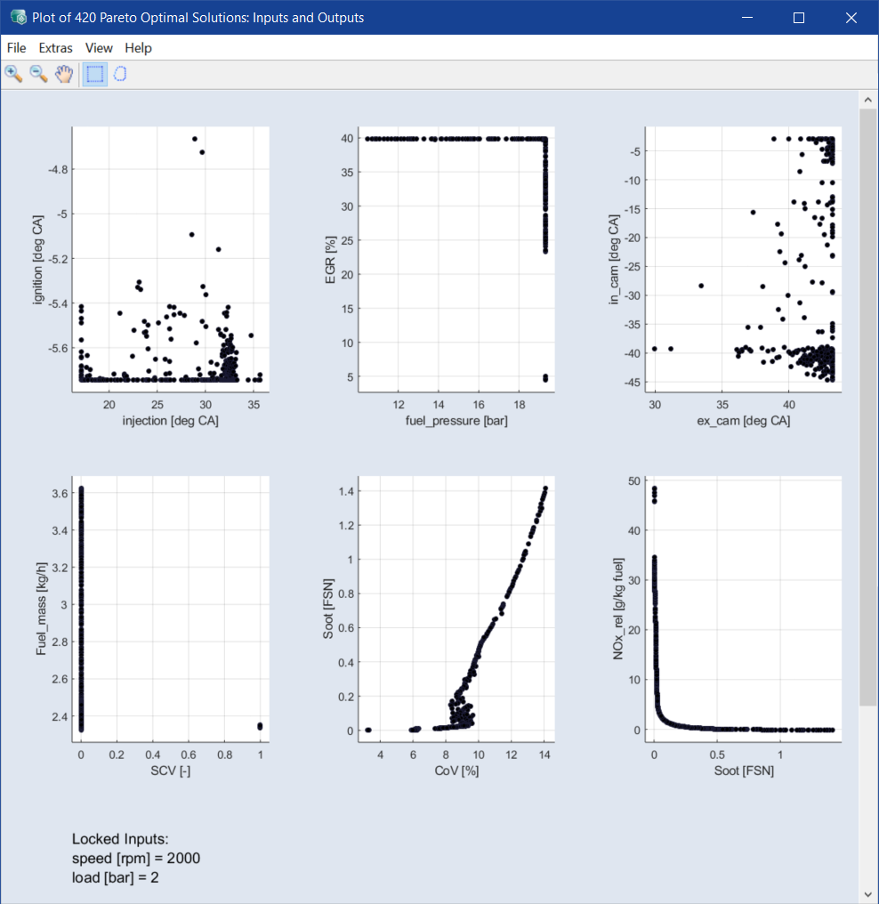
For the function of the Inputs and Outputs window, see Addressing a group of Pareto solutions.
Addressing individual Pareto solutions
-
Right-click a point of the plot (= one solution of the optimization).
The selected solution is highlighted and a context menu opens.
- Select Show Result in Other Views to display this solution in the ISP view.
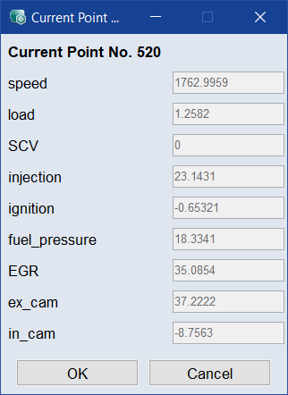
-
Select Show Result to display the values of the inputs for this solution in a window.
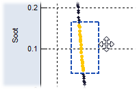
Addressing a group of Pareto solutions
- Click one of the Mouse selection * buttons.
-
Draw a rectangle or lasso around certain solutions.

The solutions inside the shape are highlighted.
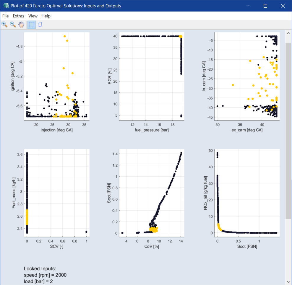
Note
These solutions are also highlighted in the other plots of the Input and Outputs windows and the concerned areas of inputs of interest can also be identified.
-
Right-click the frame.
A context menu opens with which you can perform the following actions:
-
Remove Rectangle or Remove Lasso: Removes the rectangle or lasso again and therefore the selection of identified solutions.
-
Set Position: Only available for rectangles.
Opens the Create Rectangle window where you can edit the rectangle position.
-
Mark: Marks the solutions inside the rectangle/lasso for deletion.
-
Show Number of Solutions: Displays the number of solutions inside the rectangle/lasso.
-
-
Click a side of a rectangle/lasso to move it and mark different solutions.
-
Click a corner of a rectangle to resize it.
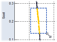
You cannot resize a lasso.
- If you are displaying additional axes with View > Select Axes, you can also observe the effect of your selection on these variables.
Saving results
You can save the entire set of Pareto-optimized solutions or solutions in a selected area in a file.
-
In one of the plot windows, select File > Export All Data / Export Intersection of Selected Data / Export Union of Selected Data.
A file selection window opens.
-
Enter a file name and click Save.
-
The solutions are saved in an Excel file.