Single-Result Optimization with Weighted Total of Single Result

The task: Minimize fuel consumption (Fuel_mass) and attempt to keep other variables, such as engine roughness (CoV), soot (Soot) and nitrogen oxide (NOx_rel), below their predefined limits.

Defining the operating point

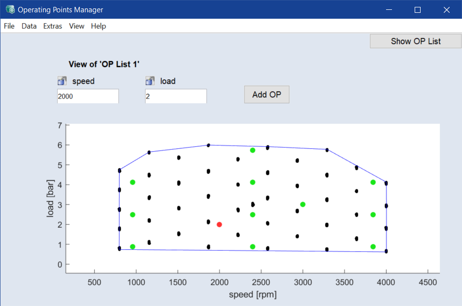
• Select In/Outputs > 2D Plot Operating Points.

  The two variables load and speed, which define the operating point, are now displayed in a separate window.

• In this window, define the operating point at which you want to perform the optimization, e.g., speed = 2000 rpm and load = 2 bar.

  

  You have to lock load and speed, or their values will be varied during optimization.

• Click the lock icons () next to speed and load.

• The locks are closed (), the input fields are disabled, and the red dot in the plot is fixed.

  

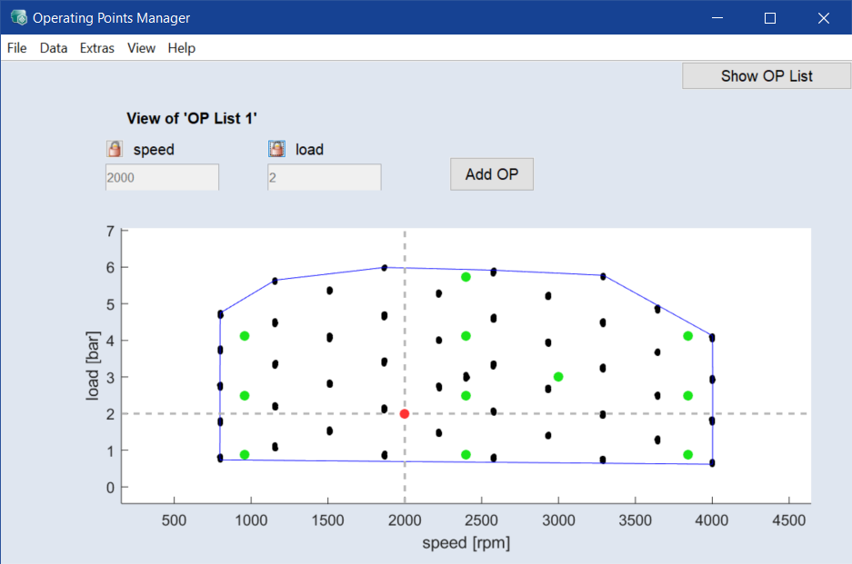
Specifying optimization variables and criteria

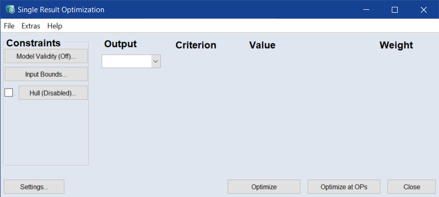
• Select Optimization > Single Result.

  The Single Result Optimization window opens. The Output column is used to select the outputs to be optimized; the other columns are used to set optimization criteria.

  

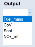
• In the Output column, click in the empty cell.

  

• Select Fuel_mass from the drop-down list.

  The respective optimization criterion is set to the default value. A new empty row is added.

• Select all remaining outputs, i.e. CoV, Soot and NOx_rel.
• Enter the following optimization criteria:

Output	Criterion	Value			Weight
Fuel_mass	Minimize	None	-	-	Constant	1
CoV	Bound	Weak Upper Bound	Constant	5 [%]	Constant	1
Soot	Bound	Weak Upper Bound	Constant	0.3 []	Constant	1
NOx_rel	Bound	Weak Upper Bound	Constant	30 [g/kg]	Constant	1

Limiting the optimization results

You can limit the optimization results to the range of valid model output in the Single Result Optimization window in different ways.

• To limit the optimization result automatically to the range of valid model outputs, do the following:

  • Click the Model Validity button.

    The Valid Model Range window opens.

  • Activate each element you want to limit to the valid model range.
  • Click OK to apply your settings and close the Valid Model Range window.

• To limit the minimal and maximal values of an input, do the following:

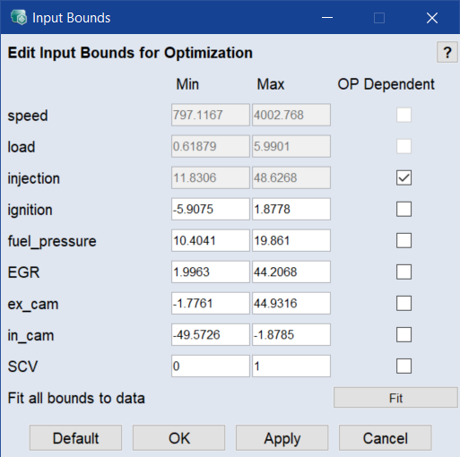
  • Click the Input Bounds button.

    The Input Bounds window opens. You can edit the min. and max. values of an input.

    

  • In the Input Bounds window, click Fit to fit all bounds to measured data.

    Or

    Do one of the following for each input you want to limit:

    • Enter the range of valid parameter variation ("Min"/"Max") for optimization.

    • Activate the OP Dependent checkbox.

      The Map Bounds window opens for the respective input. Here you can manually specify the range of parameter variation using the defined grid points.

  • In the Input Bounds window, click OK to apply your settings and close the window.

    Note
    For more information regarding the definition of valid parameter variation using OP-dependent input bounds, see Calibration .

• To limit the range of parameter variation to the data within the specified hull, do the following:

  • Activate the checkbox next to the Hull button.

    This limits the range of parameter variation to the data within the specified hull (In/Outputs > Hull on Inputs). Current setting can be checked by clicking the Hull button.

Change settings of the Single Result optimization

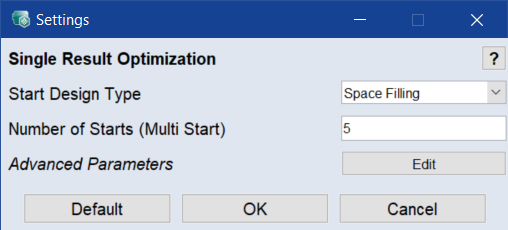
• In the Single Result Optimization window, click Settings.

  The Settings window opens.

  

  Note
  The Edit button to customize the Advanced Parameters is only available if the Advanced Settings are enabled (see Advanced Settings in ASCMO-STATIC .)

• In the Start Design Type drop-down field, specify which start design will be used for optimization.

  The following settings are possible:

  Last: The current settings in the ISP view are taken as start values.

  Space Filling: The start values are selected space-filling by Sobol algorithm.

  All Edges: Start values = all corners of the experimental space. The rest of the population is distributed in the parameter space according to the Sobol algorithm.

• In the input field Number of Starts (Multi Start), define the number of optimization runs.

  To ensure that a global minimum is found, the optimizer should be started multiple times using different start values.

• Click OK to confirm the settings.

  The settings are applied. A message appears in the log window.

Performing the optimization

• In the Single Result Optimization window, click Optimize.

• The optimization is performed.

  The results of the optimization are displayed in detail in the log window under the ISP view, and the optimized values are also set in the ISP view.

  

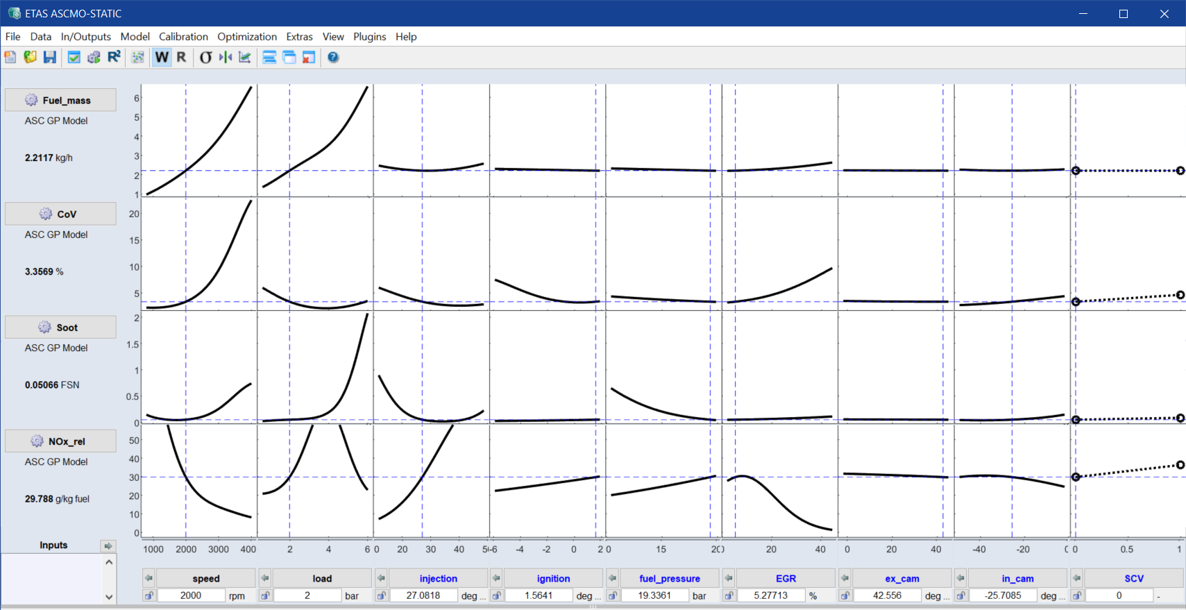
  The result manifests itself in a minimized fuel quantity while maintaining the predefined upper limits for the other outputs.

  Note
  Your results may slightly deviate from the ones achieved here since the models of the outputs may differ slightly depending on the preprocessing of the training data (removal of outliers and repetition points, etc.).

Saving the result of the local optimization

• Select Extras > Evaluation List > Add Current Settings to List to save these optimization data.

  The Model Evaluation List window opens and the current optimization result is added to it.

• In that window, select File > Export to save the Model Evaluation List for later use.
• In the Save Data file selection window, enter or select type (e.g. *.xlsx or *.xls or *.csv or *.ascii), path and name for the export file, then click Save.

Automatic optimization upon selecting the operating point

You can set up ASCMO-STATIC so that a single-result optimization is performed automatically each time you select a new operating point.

• In the operating points manager (shown in Operating points manager (A: input fields for operating point values, B: operating points, C: measurement points, D: convex hull of the plot)), select Extras > Optimize On Move.

• Click in the plot to select a new operating point (red point).

• The optimization based on the selected criteria starts for the selected operating point.