Calibration

In this section, you edit the maps obtained from the global optimization.

Note
The Calibration menu and the Global Optimization function in the Optimization menu are only available if operating point axes have been selected (see Assign Inputs and Outputs). You can set the operating point axes afterwards via the In/Outputs > Set Operating Point Axes menu option.

Viewing calibration maps

• Select Calibration > Calibration Maps > Open all Maps.

  Windows with calibration maps of all inputs obtained from the optimization open.

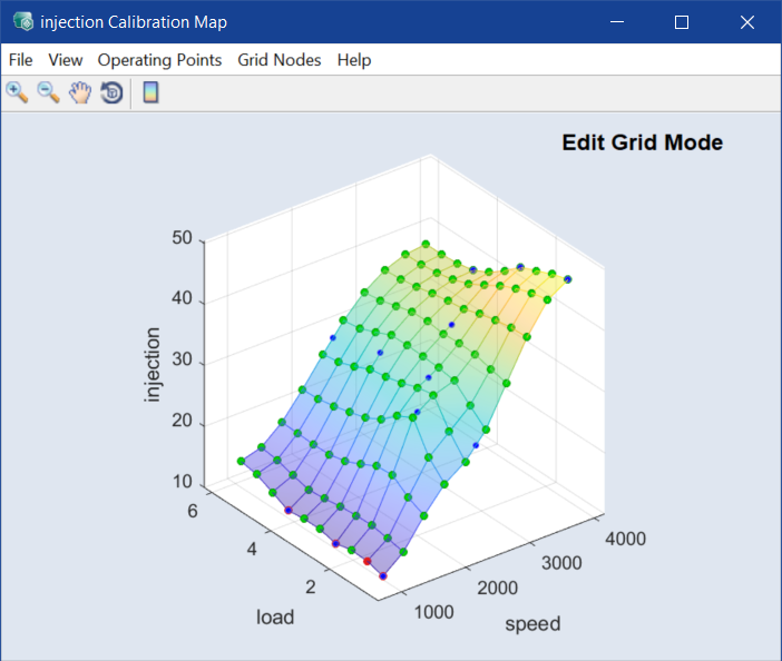
  The following figure shows the calibration map of the injection input.

  

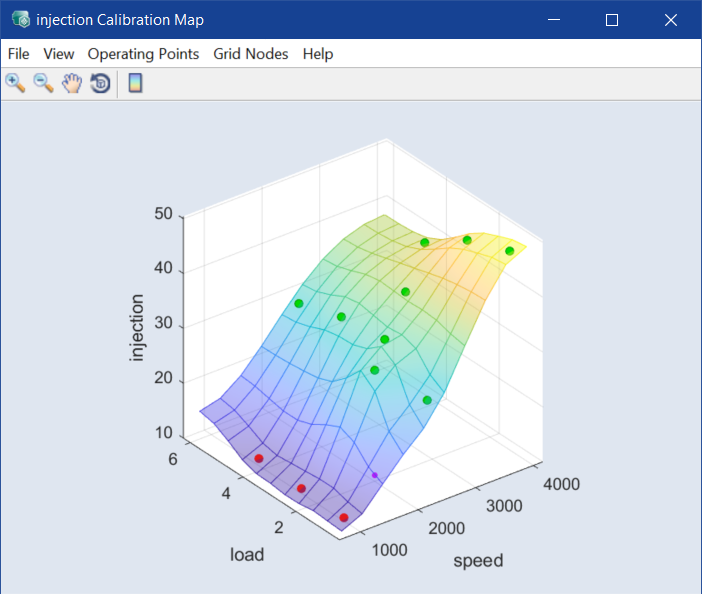
  The colored points are the operating points at which the optimization has been performed.

  • Green points indicate that the optimization result falls within the range of the measured data.

  • Points at the limit (= the smallest/largest measured value in this dimension) are marked in red.

  • Yellow is used to mark values that fall between this limit and the measuring range bounds that apply to this operating point.

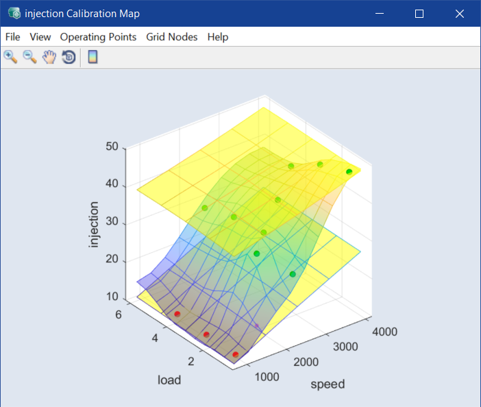
• To show the bounds of the measured range, select View > Map Bounds in a calibration map window.

  Note
  These bounds must first have been adjusted to the measured range; see Adjusting bounds to the measured range.

• The bounds of the measured range are drawn in the plot of the calibration map.

  

Adjusting bounds to the measured range

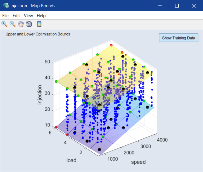
• Select Calibration > Map Bounds over OP > <input_name>, we use injection.

  The injection - Map Bounds window opens.

• Select Edit > Fit Bounds to Data.

  The Fit Map Bounds to Data window opens.

• In that window, do one or more of the following:

  • Enter a smoothness factor for the map bounds.
  • In the Grid Nodes area, redefine the grid.
  • Activate Apply to all maps to apply the changes to all <input_name> - Map Bounds maps.

• Click OK or Apply to continue.

  The areas for the lower and upper limit of the measured range of the injection input are adapted to the measured data.

  

• Close the window.

  Instead of adjusting the bounds for each input separately, you can use Calibration > Map Bounds over OP > Fit Bounds to Data or Fit Bounds to Min/Max to adjust the bounds for all inputs.

Changing values at operating points

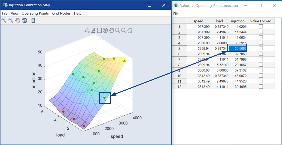
• In the injection Calibration Map window, select Operating Points > Table of Values at OPs.

  The Values at Operating Points: injection window opens.

• In the injection Calibration Map window, click one of the operating points marked in color and hold the mouse button pressed.

  The mouse pointer changes to a double arrow. At the same time, the cell with the corresponding value is marked in the table.

  

• Now, move the point with the mouse.

  The value of injection is also changed in the table (and in the ISP view).

• In the Values at Operating Points: injection window, change a value of injection at another operating point and press <Enter>.

• The plot and (if View > Update ISP Online is activated) ISP view are adjusted accordingly.

  You can also make predictions of how these changes will affect a predefined driving cycle.

Opening the prognosis window

• Select Calibration > Prognosis > Results.

  The Prognosis Results window opens.

  

• Move a point in the injection Calibration Map window, as shown in Changing values at operating points.

  The effects of this change on the outputs can be seen directly in the Prognosis Results window.

Adjusting grid nodes

• To render the display of the injection map more clearly, deactivate View > Map Bounds in the plot window.

• Select Grid Nodes > Grid Nodes > Define Grid Nodes.

  The Change Grid Node Vectors window opens.

• To change the number of grid nodes in a calibration map, do the following:

  • Enter the desired values in the Count fields.

    

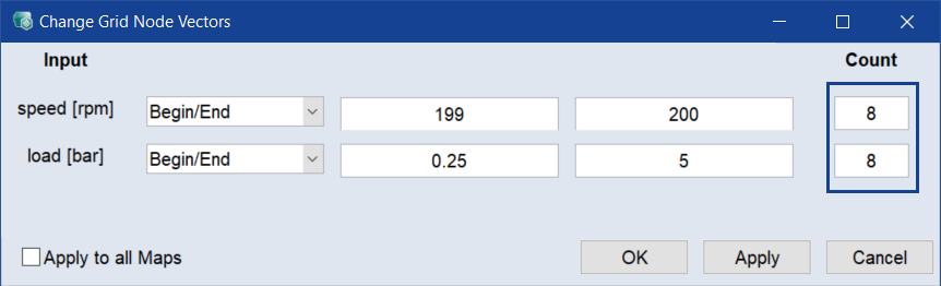
  • Click Apply.

    The 10 x 10 grid for the grid nodes of the map is drawn. The values on each axis are equidistant.

  Or

  To enter the grid vectors directly, do the following:

  • In the drop-down list for each input, select Support Vector.

    The vectors of the grid nodes are displayed in the field of the corresponding input map.

  • If necessary, edit the vector values and click OK.

    The grid nodes of the map are adjusted accordingly. The Change Grid Node Vectors window closes.

    Note
    When you add/edit a vector (Support Points), the number of nodes in the column Count is adjusted automatically.

Editing the map

• In the injection Calibration Map window, select Grid Nodes > Edit Grid.

  Similar to the optimized values of injection at the operating points, the (interpolated) values at the selected grid nodes of the map are now marked by colored points. The operating points, at which optimizations have been performed, are also displayed (small points).

  

• To save the original state of the map, select File > Set as Reference Page.
• The values at the grid nodes can now be edited as described in Changing values at operating points.
• To reset the state of the map to the optimization result, select File > Reset from Reference Page.

Saving the calibration map

Finally, you can export the optimized and, if necessary, edited map.

• In the injection Calibration Map window, select File > Export.

  A file selection window opens in which you can save the map as DCM file (*.dcm) or in CSV format (*.csv). The default file name is <project_name>_CM_Injection.*.

• In the following window, enter a label name and click OK.

  

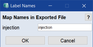
• The map is saved.