Optimization at Several Operating Points

The method described in Single-Result Optimization with Weighted Total of Single Result can also be executed in a type of batch mode. The optimizer sequentially runs through a series of operating points, thereby optimizing "globally".

This optimization is the starting point for creating maps based on modeled outputs.

Defining the grid of operating points

First, select the points at which you want to optimize.

• Select Calibration > Operating Points.

  The Operating Points Manager window (see Operating points manager (A: input fields for operating point values, B: operating points, C: measurement points, D: convex hull of the plot)) opens.

• In that window, select Data > Edit List > Redefine Grid to create a grid that deviates from the default.

  The Redefine Grid for OP List <n> window opens.

• In that window, do the following:

  • In the drop-down lists of both parameters, select Begin/End
  • In the input fields, enter the ranges for speed and load.

  • In the Count column, enter, e.g., a 5x5 grid.

    

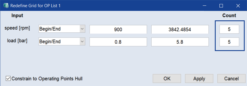
  • If desired, activate the Constraint to Operating Points Hull option to ignore operating points outside the hull.

  • Click OK to apply your settings and close the window.

    A 2-dimensional grid of equidistant points is created. The points are shown in the operating points manager.

  It is also possible to import an existing list of operating points via File > Import in the operating points manager.

Defining optimization criteria

• Select Optimization > Single Result.

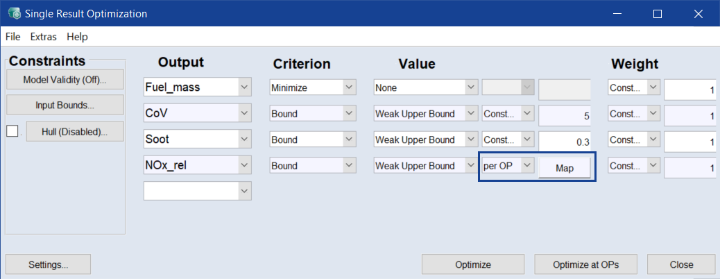
  The Single Result Optimization window opens. The window contains the criteria of the previous local optimization.

• For the NOx_rel output, change the value in the middle Value column from Constant to per OP.

  The input field in the right Value column becomes a button.

• Click Map.

  

  The plot for the optimization settings at all defined operating points opens.

  

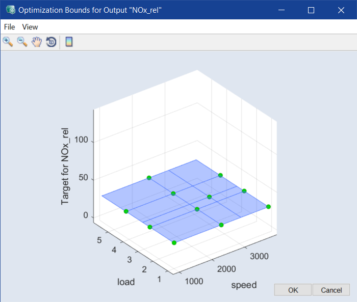
  The value 30, which was previously the default for the Constant setting, has been copied to all operating points.

• To edit the value of a single operating point, do one of the following:

  • Move a point with the mouse.

  • Select View > Table, then edit the values in the Optimization Target Table for Output * window.

• If desired, select File > Import Target Map to load an Excel file with the settings (values at the respective operating points).
• To continue with this tutorial, close the window with Cancel to discard any changes you made.

Performing the optimization at all operating points

• In the Single Result Optimization window, click Optimize at OPs.

  The optimization is performed.

  A window opens in which you can track the progress of the optimization at the individual operating points.

  

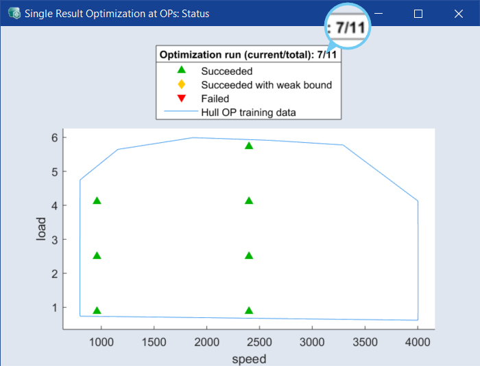
  During the optimization at the respective operating points, the optimization values are set in the ISP view and output in the status window.

  The optimization was successful at the green operating points.

• To represent the results of the optimization runs at the operating points in a table, select Extras > Optimization at OPs >Show Results in the Single Result Optimization window.

  The Optimization Results window opens. It contains the optimized results for all operating points.

  

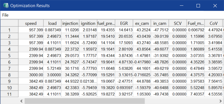
  In addition, the table contains the standard deviations at the respective operating points.

• In the Optimization Results window, mark a row and select File > Show Current Row in Intersection Plot.

• The values of the inputs and (as a result) the outputs are set in the ISP view.

  This list can also be saved as Excel file (File > Export).

Transfer optimization results to Calibration Maps

• In the Optimization Results window, select File > Apply Results to Calibration Maps.

• In the main menu, select Calibration > Calibration Maps > * to view the new calibration maps.

  Note
  For more information on handling and visualizing calibration maps, see Calibration .

Viewing optimization results (Result Maps)

• Select Calibration > Result Maps > Open all Maps.

  The plots of the results for all outputs are opened.

  
  

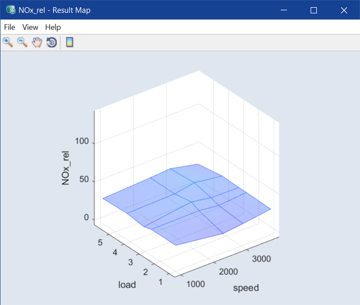
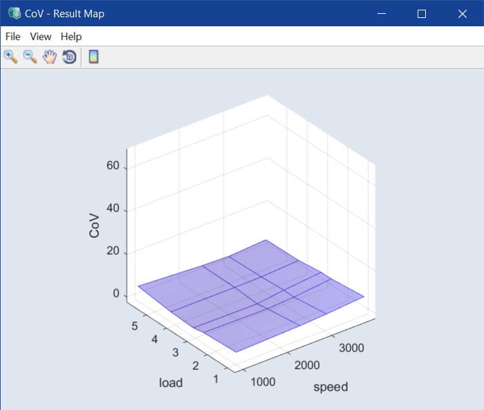
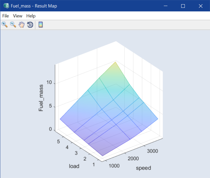
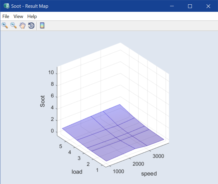
  The points represent the operating points at which the optimization has been performed.

• In the main menu, select View > Close Child Windows to close the plot windows and any other child windows.

Note
The current results of the optimization – the maps – are described in section Calibration .