Calibration Menu
|
Note |
|---|
|
The Calibration menu is only available if operating point axes have been selected. You can set the operating point axes via the In/Outputs → Set Operating Point Axes menu option (see Set Operating Point Axes). |
The Calibration menu consists of the following entries:
- Operating Points
- Driving Cycles
- Calibration Maps
- Map Bounds over OP
- Map Viewer & Converter
- Result Maps
- Result Value Table
- Prognosis
Operating Points
Opens the "Operating Points Manager" window.
Driving Cycles
Opens the "Driving Cycle Manager" window.
Driving cycles are produced by different countries and organizations to assess the performance of vehicles in various ways, as for example fuel consumption and polluting emissions. Another use for driving cycles is in vehicle simulations. More specifically, they are used in propulsion system simulations to predict performance of internal combustion engines, transmissions, electric drive systems, batteries, fuel cell systems, and similar components.
Calibration Maps
The Calibration Maps sub menu contains the following options:
-
<n: input>
Opens the "<input> Calibration Map" window that shows the map of the selected input gained from the optimization at several operating points.
-
Open all Maps
Opens "<input> Calibration Map" windows for all calibration maps gained in the optimization.
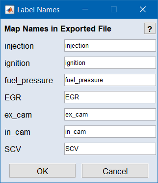
-
Saves the maps of all inputs as DCM, CDFX or CSV file. First, you can assign names for the labels.
-
Import
Allows loading maps that are present as DCM, CDFX, CSV, Excel or ASCMO project files and editing them in the project. First, the individual labels in the file must be assigned to the inputs of the current project.
-
The calibration map selected via the sub menu options (<n: input> and Use All Maps) is used as input. The input is then highlighted with red font in the ISP view.
-
Sets all working maps active.
-
Use Reference Page
Sets all reference maps active.
-
Sets all working maps as reference maps.
-
Reset Maps from Reference Page
Resets all working maps to maps previously set as reference.
The working map or reference map is displayed here depending on the selection (in the toolbar of the main window or via Calibration → Calibration Maps → Use Working Page/Use Reference Page). Setting a current working map as reference and resetting a map that has possibly been edited as reference takes place via File → Set Reference Page and File → Reset from Reference Page).
|
Note |
|---|
|
The calibration map set as reference can no longer be edited. |
Application example: The calibration map gained from optimization is set as reference - after further optimization (with for example a different weighting of the optimization criteria), a comparison can be made between the two results.
|
Note |
|---|
|
This also particularly applies to the representation of the results in the prediction. |
Map Bounds over OP
The range of the measuring data can be assigned an upper and a lower bounds area whose base points are determined by the currently defined grid of operating points.
This bound is important for the optimization and subsequent display of the maps (Calibration > Calibration Maps).
-
<n: input>
Opens the plot with the measuring data of the respective input and the currently specified bounds areas for these data (see The "<input> - Map Bounds" window).
-
Open all Bounds
Opens all plots with the measuring data and the currently specified bounds areas for these data (see The "<input> - Map Bounds" window).
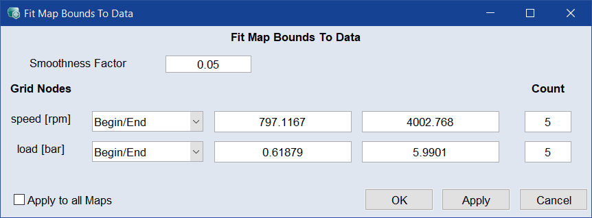
-
Fit Bounds to Data
Fits the bounds of the current map to the measured data via the
 "Fit Map Bounds To Data" window.
 -
Fit Bounds to Min/Max
Sets the bounds to the highest and lowest point of the measurement data.
-
Export All Bounds
Exports all Bounds to a file (*.dcm/*.cdfx/*.csv).
-
Import All Bounds
Imports all Bounds (upper/lower) from an already existing file (*.dcm/*.cdfx/*.csv/*.xls/*.ascmo).
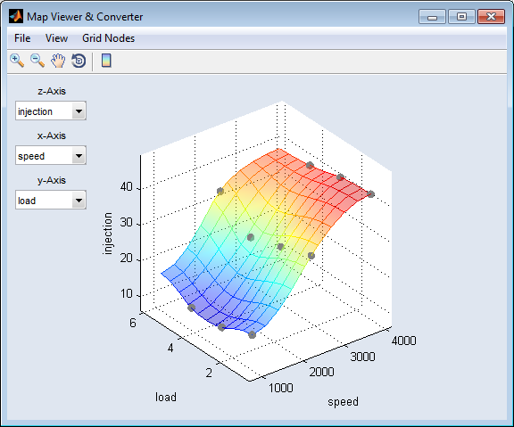
Map Viewer & Converter
Opens the "Map Viewer & Converter" window where you can display and export map plots. Both inputs and outputs can be selected as axes - the data of the Result Value Table is displayed.
- File → Export...
Saves the Calibration map as DCM or CSV file (<project name>_CM_<input>.*). First, you can assign a name for the label. - File → Close
Closes the "Map Viewer & Converter" window. - View → Save as Bitmap...
Allows saving the plot in a series of graphic formats. - View → Copy to Clipboard
Copys the plot to the clipboard. - View → Visible Z-Range
Allows adjusting the Z axis of the plot. - View → Show Toolbar
Allows showing and hiding the toolbar. - View → Prepare Print
Opens the "Prepare Print Options" window where you can adjust the look of the plot area. The settings are reset when you close the plot window. - View → Contour Mode
Allows showing and hiding the contour lines in the 3D-Plot. - Grid Nodes → Load Grid
Allows loading grids from a file (*.dcm, *.csv or *.xls). - Grid Nodes → Define Grid Nodes
Allows defining the values and the number of grid nodes for a new grid.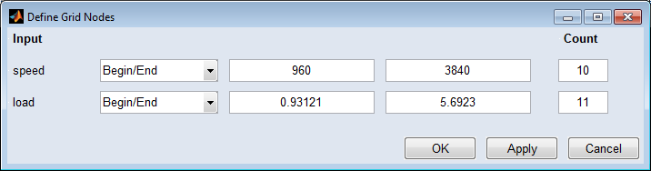
- Grid Nodes → Set to Operating Points
Allows adopting the grid of the operating points at which optimizations were performed as base point grid. - Grid Nodes → Table
The result map displayed in the plot window is displayed as a table. The values of the table can be saved via the File → Save Table... menu. - Grid Nodes → Smoothing
A slider editor appears in the plot window with which you can smooth the map (not in "Edit Grid" mode).
The toolbar of the window contains the following elements:

|
Zoom In | Clicking in the plot will enlarge the plot representation. |

|
Zoom Out | Clicking in the plot will reduce the plot representation. |

|
Pan | Thus, the plot can be shifted within the window. |

|
Rotate 3D | Thus the 3D plot can be rotated in all three spatial directions. |

|
Insert Colorbar | Displays the current color table with the axis scaling. |
Result Maps
The Result Maps sub menu contains the following options:
-
<n>: <output>
Opens the "<output> Result Map" window for the selected output.
-
Open All Maps
Opens the result maps of all outputs.
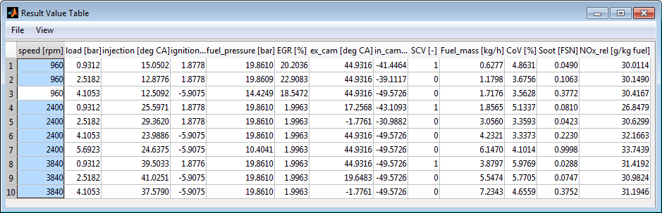
Result Value Table
Opens the "Result Value Table" window that shows a table with the optimization results (for inputs as well as outputs) at all operating points at which an optimization was performed.
Prognosis
With the results gained from an optimization, prognoses can be represented here, e.g. about consumption or emission quantities.
-
Opens the "Calculation Rules for Prognosis" window. To adjust the values of model outputs to known parameters and to certain driving cycles, conversions and weightings are performed here.
-
Opens the "Prognosis OP-Weights" window.
With the weighting of the duration of stay at certain operating points, you can map a driving cycle. The weights of the operating points can also be calculated by measuring a trajectory. This involves each measurement being assigned to an operating point and totaled which in turn results in the weighting for each of the operating points defined previously.
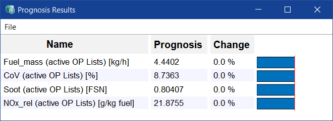
-
Opens the
"Prognosis Results" window where the effects of changes in the prognosis parameters (Prognosis → Calculation Rules) and/or to maps on outputs are displayed.