|
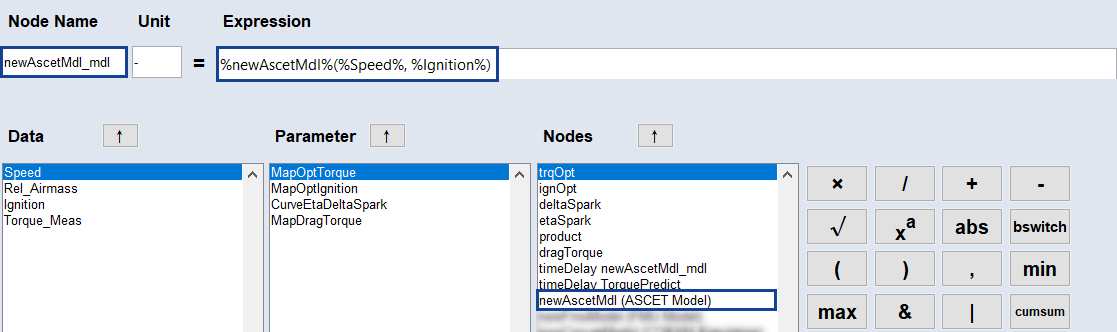
Inserts the *, /, +, or - operator into the expression.
This results in element-wise multiplication, division, addition, or subtraction.
|

|
Inserts the square root sqrt( operator into the expression. The expression must end with )..
|

|
Inserts the ^ operator into the expression.
x^y means row-by-row x to the power of y.
|

|
Inserts the absolute value abs( operator into the expression. The expression must end with ).
Example abs(-3) ≥ 3 abs(-3) ≥ 3
|

|
Inserts the bswitch( operator into the expression. The expression must end with ).
Binary switch, element-wise:
y = bswitch (x, a, b)
y = a for x <= 0
y = b for x > 0
Examplebswitch (%speed% > 2000, %Y_1%, %Y_2%)
|
|
Inserts an opening or closing bracket into the expression.
|

|
Inserts a comma into the expression.
|
|


|
Inserts the min(/max( operator into the expression. The expression must end with )..
min = minimum of two inputs
max = maximum of two inputs
Examplemin(%in1%, %in2%), max(%in1%, %in2%)
|
|

|
Inserts the & operator into the expression, which means a logical element-wise AND.
Example%Speed% > 2000 & %Load% > 6
|
|

|
Inserts the | operator into the expression, which means a logical element-wise OR.
Example%Speed% > 2000 | %Load% > 6
|
|

|
Inserts the ~ operator into the expression, which means a logical not.
Example
~(%x1% & %x2%)
|
|

|
Inserts the cumsum( operator into the expression, which means the cumulative sum of a numerical sequence. The expression must end with ).
Examplecumsum(%y%): [1 2 4] ≥ [1 3 7]
|
|


|
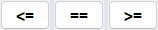
Inserts the </<=/==/>=/> operator into the expression, which means is less than/less than or equal to/equal to/greater than or equal to/greater than.
|

|
Inserts the warnif( operator into the expression. The expression must end with ).
It allows you to define checks that are automatically executed after each optimization run. If the defined condition is met, the specified warning text is displayed in the log window.
To use the warnif operator, you need to insert a condition in the expression field after clicking the button. The syntax for the warnif operator is as follows:
y = warnIf(condition, 'warningText').
Examples
warnIf(%MapDragTorque%(%Speed%, %Rel_Airmass%) > 0, 'Warning')
In this example, if at least one of the values of the map parameter MapDragTorque is greater than zero after the optimization, the text "Warning" will appear in the log window.
warnIf(%speed% < 0, 'speed less than zero')
In this case, if the value of speed is less than zero after the optimization run, the warning "speed less than zero" will be issued.
|
|

|
Inserts the timeDelay( operator into the expression. The expression must end with ).
It allows you to delay a signal by one time step. After clicking the button, you need to insert a condition in the expression field using the following syntax:
timeDelay(x, initialValue)
In this expression, initialValue is returned in the first step, and it is the only way to access nodes further in the function.
Examples
timeDelay(%transferFcn%, %setpoint%(1))
In this example, the signal from transferFcn is delayed by one time step, with the initial value set to the first element of the input setpoint.
y = timeDelay(%y%, 0.0)
Here, the value of y is delayed by one time step, with an initial value of 0.0.
|
|

|
Inserts the delta T (sample time, dT) operator into the expression.
It represents the sample time in the data and will be replaced with the corresponding value during execution.
Examples
dT ./ %filterConstant%
In this example, dT is the value from the time [s] column in the Data step, while %filterConstant% is a parameter used in the calculation.
y = timeDelay(%y%, 0.0) * dT
In this case, the value of y is multiplied by the sample time dT after applying a time delay.
|
|

|
Inserts the roundToDiscreteValues( operator into the expression, which rounds a node to a specific discrete value. The expression must end with ).
After inserting the operator, you need to select a discrete parameter and enter the desired values. The syntax is as follows:
roundToDiscreteValues(node, [value1, value2, ...])
Examples
roundToDiscreteValues(%calMap_SCV%(%speed%, %load%), [0, 1])
In this example, the output of the calibration map calMap_SCV is rounded to the discrete values 0 and 1 based on the inputs speed and load.
roundToDiscreteValues(%myTernary%, [0, 1, 2])
Here, the value of myTernary is rounded to the discrete values 0, 1, and 2.
|
|

|
Inserts the steadyState_abs( operator into the expression, which calculates the steady state of a signal based on the window length and window height. The expression must end with ). The syntax is as follows:
steadyState_abs(x, windowLength, windowHeight, sampleRate)
Example
steadyState_abs(%signal%, 10, 200, dT)
In this example, the steady state of the signal is calculated using a window length of 10, a window height of 200, and the sample rate represented by dT.
|
|

|
Deletes the last entry in the expression field (backspace).
|
|
The following operators are supported. Select them from the burger menu ( ) or type them in manually: ) or type them in manually:
|
|
log(x)
|
The natural logarithm (base e).
Examplelog(exp(2)) => 2
|
|
log10(x)
|
The common logarithm (base 10).
Examplelog10(10^2) => 2
|
|
exp(x)
|
Euler's number raised to the power of ex.
Exampleexp(1)) => 2.718
|
|
sin(x), cos(x), tan(x), tanh(x), atan(x)
|
The trigonometric functions, the input is in radians.
Examplesin(3.1416) ~> 0
|
|
atan2(x, y)
|
The four-quadrant inverse tangent, input is given in radians.
Exampleatan2(%id%, %iq%)
|
| delayseq(data, n)
|
Delay a signal by n time steps. The start of the signal is filled with zeros.
Exampledelayseq([1; 2; 3; 4;], 2) => [0; 0; 1; 2]
|
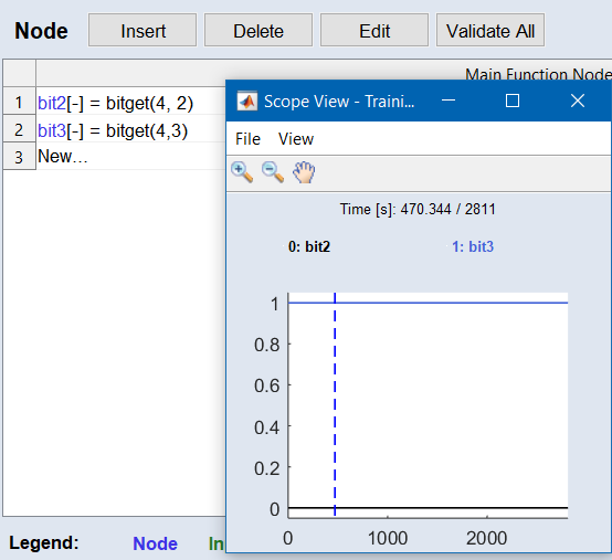
| bitget(x, bitPos)
|
The MATLAB® bitget function returns a bit value at a specified position (bitPos).
Example
bitget(4, 3) returns 1
bitget(4, 2) returns 0
In this example, the integer 4 is represented in binary as 100. The function bitget(4, 3) retrieves the bit at position 3, which is 1, while bitget(4, 2) retrieves the bit at position 2, which is 0.
|
|
Further notations are supported:
|
|
z = [x, y]
|
Creates a multidimensional vector. A vector can be extracted with y = z(:, 2). This can be useful, e.g., when a subfunction shall returns multiple nodes/vectors.
|
|
y = zeros(size(x))
|
Creates a vector of zeros.
|
|
y = ones(size(x))
|
Creates a vector of ones.
|
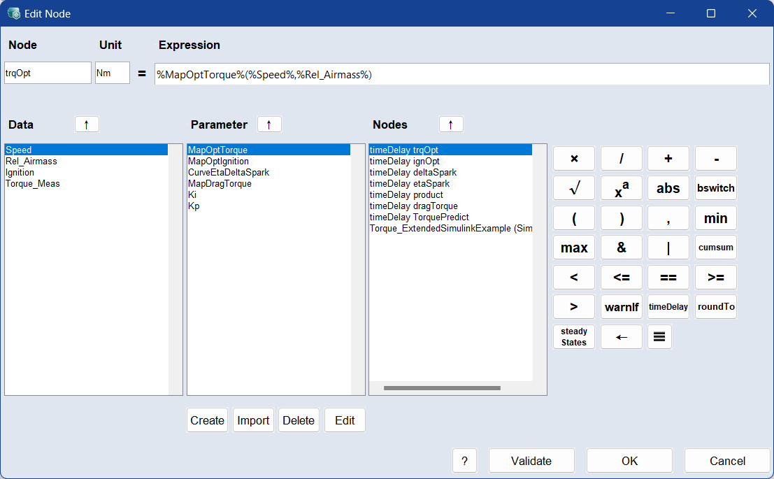
 Insert Data into Formula
 Create