Intersection Plot (ISP)

The modeled dependencies of the output variables on the inputs are visualized using intersection plots. General information about the intersection plots is given in Intersection Plots .

Loading the project

If you saved a previously processed ASCMO-STATIC project, you can continue working with it. To do so, proceed as follows.

• Do one of the following:

  • In the ASCMO-STATIC start window: click Open ASCMO Project.
    (cf. Starting ASCMO-STATIC )
  • In ASCMO-STATIC user interface: click File > Open.
    (cf. Elements of the ASCMO-STATIC User Interface)

• In the file selection window, select the project file (*.ascmo) and click Open.

• The project opens.

Scaling axes

In principle, the scaling for the Y axes (= outputs) is determined automatically. However, this scaling can also be changed manually.

• Right-click in a plot.

  A context menu opens. The Autoscaled Output Range <output> option is enabled by default.

  

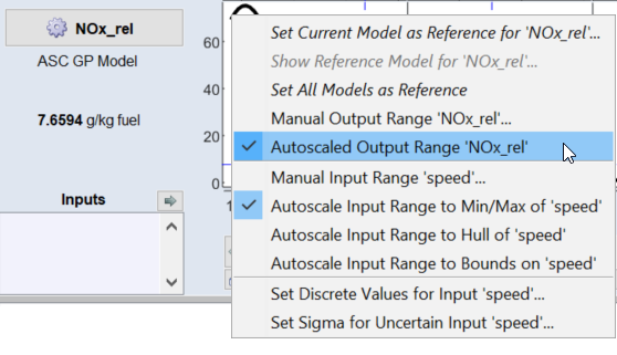
• Select the option Manual Output Range <output>.

• A window for entering the range to be displayed opens.

  

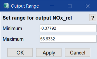
• Enter minimum and maximum, then click Apply or OK.

The display range of the inputs can be scaled manually or automatically using the context menu options (right-click in the intersection plot) Manual Input Range * and Autoscaled Input Range *.

Defining the display of inputs

• Select In/Outputs > Input Properties.

• In the Input Properties window, activate the Show checkbox for all inputs you want to display.

  

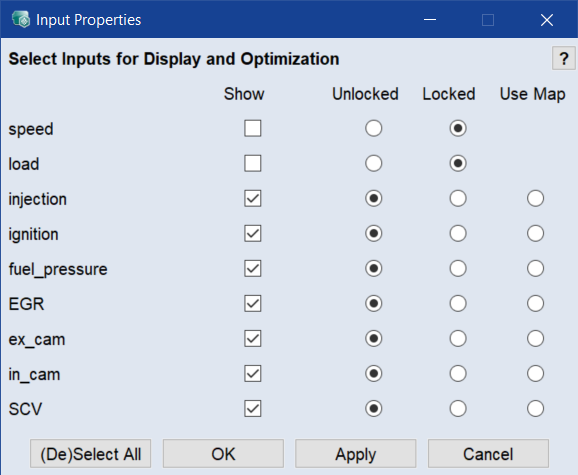
  Since only unlocked inputs are optimized, it is recommended that you keep the default setting unlocked for all inputs in this tutorial.

• Click OK.

  Intersection plots for the non-selected inputs are no longer displayed. Instead, the inputs are listed at the bottom left.

  or

  As an alternative, click the arrow next to an input name to deactivate this input.

  

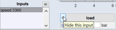
• Double-click an entry in the Inputs list to re-enable that input or select multiple inputs with strg/ctrl and use the arrow.

Setting values of inputs

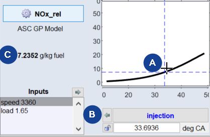
• Setting a value (A)

  To set an X value in an intersection plot, click a point.

  To continue navigating, hold the left mouse button pressed, drag the cross in the plot, and release the mouse button again at the desired point (A).

• Current value of the respective input (B)

  The value of the input can also be entered directly in the field under the name of the input.

• Current value of the output (C)

  The corresponding output value is also displayed. The shapes of all other plots are adjusted accordingly.

Optimizing manually and storing the results

You can manually perform simple optimization tasks:

• Select In/Outputs > 2D Plot Operating Points to display the operating points in the Operating Points Manager window.

  Operating Points Manager opens (see Operating points manager (A: input fields for operating point values, B: operating points, C: measurement points, D: convex hull of the plot)).

• Enter 3000 and 3 in the input fields to set speed to approx. 3000 and load to approx. 3.

• Adjust all inputs so that the value of the Fuel_mass output becomes as small as possible.

  From the intersection plots for the Fuel_mass output, it can be seen immediately that the inputs injection and EGR will have the greatest influence on the fuel consumption.

• After you have established the desired settings (Fuel_mass should be approx. 4), select Extras > Model Evaluation List > Add Current Setting to List in the main menu.

  The Model Evaluation List window opens and the values currently set in the ISP view are copied into the list.

  

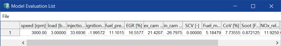
• Optionally: Save the list via File > Export.