Constraint Types "Map" and "Curve"

Selecting variables

• In the Show column, activate the checkbox for the constraint you want to edit.

  The constraint is displayed in the lower part of the window. The drop-down lists x-Axis and y-Axis (and z-Axis for maps) are provided.

• In the drop-down lists, assign the relevant inputs to the axes.

  In the case of a curve, the functional dependency is y(x); in the case of a map, the functional dependency is z(x,y).

Graphical Display of Preliminary Values and Constraint

If a completely specified constraint is selected in the list, the measurement points of the current experiment plan are displayed in a 2D (Curve, see ASCMO-DYNAMIC ExpeDes Step 2: Constraints (Type Curve)) or 3D plot (Map).

The display of the preliminary values is controlled via the Preliminary Values checkbox (region D in ASCMO-DYNAMIC ExpeDes Step 2: Constraints (Type Curve)). Only a part is shown to ensure a smooth operation. In addition, the thicker points of the grid with which the constraint of areas is controlled are also displayed.

Constraining the measurement range

• In the Show column, activate the checkbox for the constraint you want to edit.

  The constraint is displayed in the lower part of the window.

• In the constraint plot (region C in ASCMO-DYNAMIC ExpeDes Step 2: Constraints (Type Curve)), click a point of the constraining line/area and hold the mouse button pressed.

  The mouse pointer changes to a double arrow.

• Drag the point to the desired position.

  The figure shows a limitation of the torque at lower speeds.

  

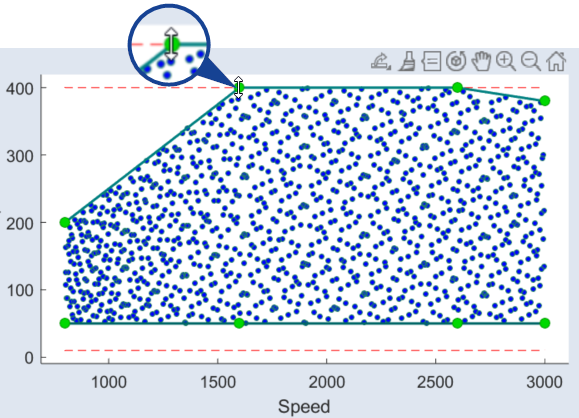
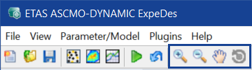
The display of the plot can be influenced here with the Zoom In, Zoom Out, Pan and Rotate 3D buttons in the toolbar.

The numeric values of the constraining points are shown in the tables on the right (Upper and Lower tabs; region E in ASCMO-DYNAMIC ExpeDes Step 2: Constraints (Type Curve)) and can be processed in these (both in terms of quantity and value); see section Table for Displaying and Editing the Grid Nodes.

Further functions for specifying and displaying constraints are.

• Display Options

  • Preliminary Values: Display of preliminary values calculated by all defined constraints

  • Upper/Lower: Display of the upper/lower limits defined by the constraint

• Time Dependence: The options and fields in this area can be used to constrain the value range or gradient range of a variable as a function of time. See the online help for details.

Table for Displaying and Editing the Grid Nodes

The grid nodes can be edited in the tables to the right of the plot (region E in ASCMO-DYNAMIC ExpeDes Step 2: Constraints (Type Curve)). One tab each is available for the upper and lower constraint.

Changing the number of grid nodes

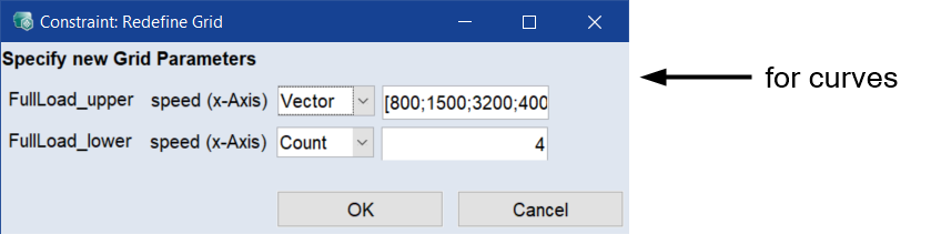
• Click Redefine Grid.

  The Constraint: Redefine Grid window opens.

  
  

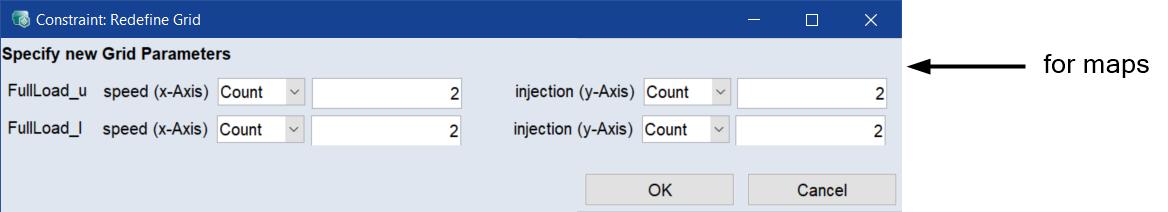
• To change the number of points on a constraint axis, do the following:

  • In the drop-down list for the constraint axis, select Count.

    The number of points is displayed in the input field for the respective constraint axis.

  • Enter the desired number.

• To enter the grid vector for a constraint axis directly, do the following:

  • In the drop-down list for the constraint axis, select Vector.

    The vector is displayed in the input field for the respective constraint axis.

  • Edit the vector values as desired.

    Note
    With type Count, the grid points are equidistant. With type Vector, you can distribute the grid points unevenly.

• Click OK.

  The points are adjusted accordingly. The Constraints: Redefine Grid window closes.