Step 2: Constraints
This step deals with constraints of the measurement range of a variable as a function of other variables. For example, it may be desirable to avoid high loads in case of high rotational speeds.
The following constraint types are available:
- Curve/Map – the value range of a variable is constrained by a function of one (Curve) or two (Map) other variables
- Time Exp. Value – the value range of a variable is constrained by a function of time
- Time Exp. Gradient – the gradient range of a variable is constrained by a function of time
In the "Constraints" Step, these conditions can be added (also imported), visualized, configured and deleted again.
Adding constraints
Clicking on Add adds a new row to the list. The following information is required for the specification:
- Constraint Name
Name of the condition to be constrained - Constraint Type
Map, Curve, Time Expansion Value, Time Expansion Gradient
Showing/selecting constraints
Via selection in the Show column, the selected constraint is shown and editable in detail.
Activating/deactivating constraints
Via selection in the Active column, the selected constraint is activated or deactivated.
Sorting constraints
With the Move Up  and Move Down
  buttons you can change the order of the constraints in the list. This order determines the order in which the constraints are processed.
Deleting constraints
Clicking on Delete removes the selected row.
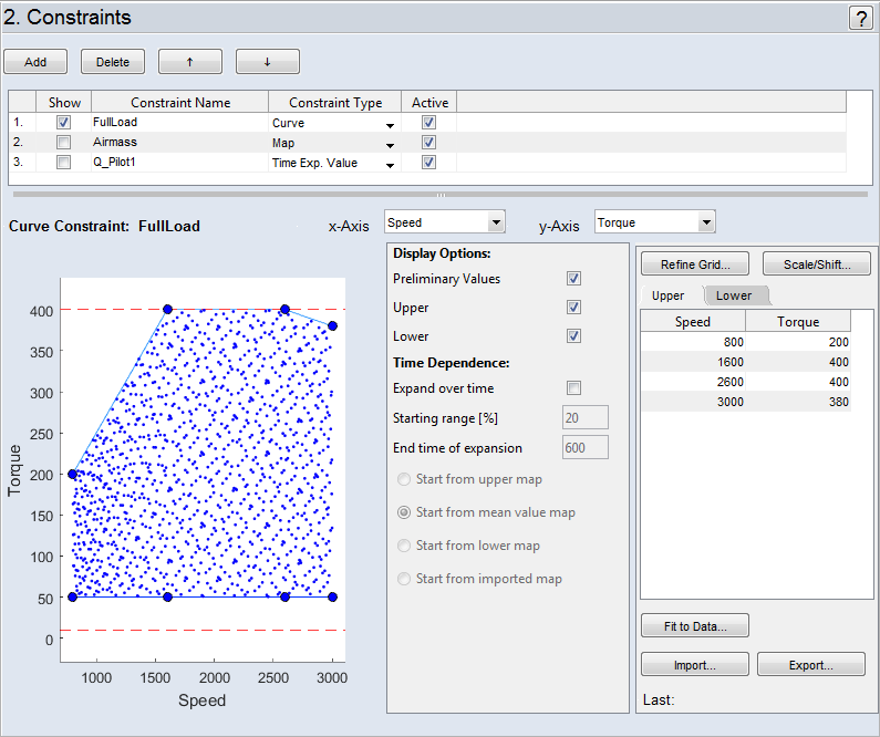
Constraint Type "Map/Curve"
This area contains the graphic display of the planed measurement points and the specified limitation of the area.
Selecting variables
Assign the relevant inputs to the axes. In the case of a "curve" the functional dependency is "y(x)", in the case of a map "z(x,y)".
The measurement points of the current experiment plan are displayed in a 2D (or 3D) plot. The display of the preliminary values is controlled via the Preliminary Values option within the "Display Options" area. Only a part is shown to ensure a smooth operation.
In addition, the thicker points of the grid with which the constraint of areas is controlled are also displayed.
- Click on a point of the constraining line/area.
- The mouse pointer changes to a double arrow.
- Hold the mouse button pressed and drag the point to the desired position.
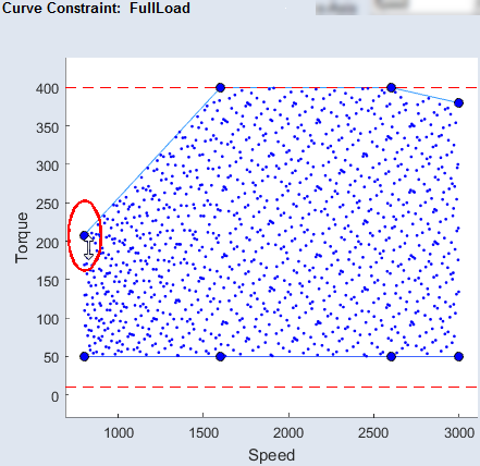
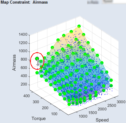
The display of the plot can also be influenced here with the tools of the toolbar (zoom, pan and rotate).
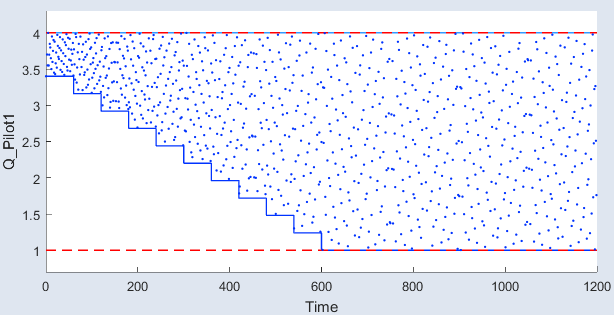
Constraint Type "Time Exp. Value/Time Exp. Gradient"
This area is only adapted to determine the extent of the input values manually.
Selecting variables
Assign the relevant input to the axis. The functional dependency is "y(time)".
The measurement points of the current experiment plan are displayed in a 2D plot. The display of the measurement points is controlled via the "Preliminary Values" option within the "Display Options" area.
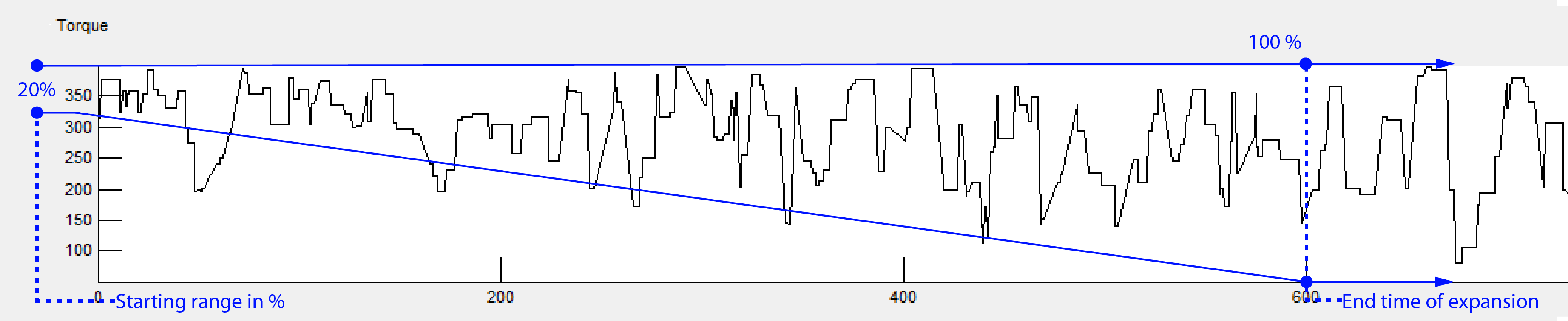
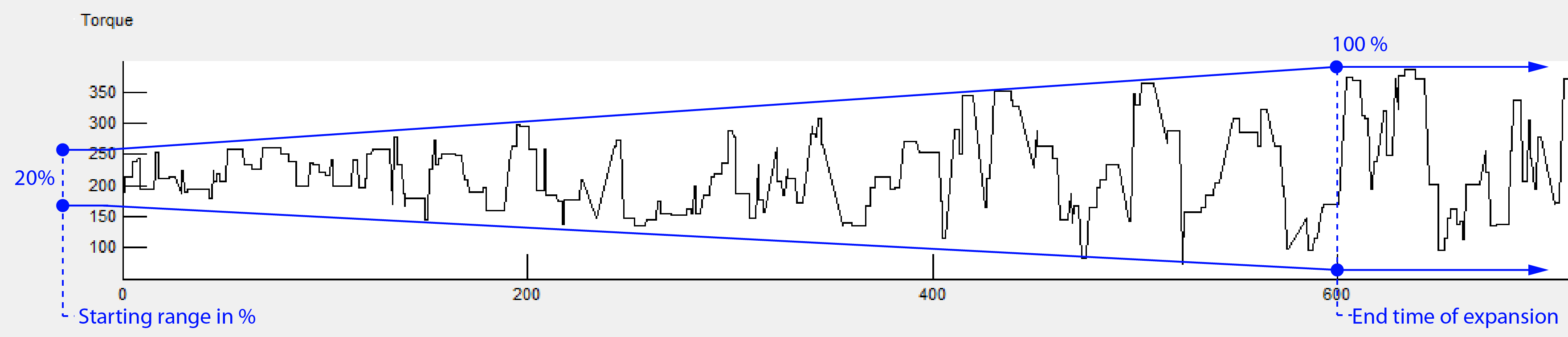
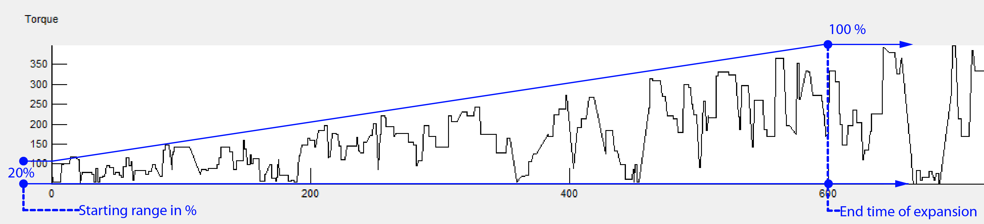
Starting range [%]
Here you can set the reach of the measurements points from where the expansion starts.
End time of expansion
Here you can set the time when the measurements are completely expanded.
Start from upper map
The expansion occurs from the upper limit towards the lower limit.
The display of the plot can be influenced with the Zoom * and Pan buttons of the toolbar.
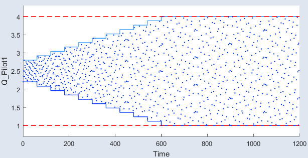
The expansion is based on the mean value of the upper and lower limit and extends in both directions.
The display of the plot can be influenced with the Zoom * and Pan buttons of the toolbar.
Start from lower map
The expansion occurs from the lower limit towards the upper limit.
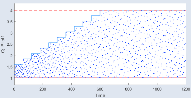
The display of the plot can be influenced with the Zoom * and Pan buttons of the toolbar.
|
Note |
|---|
|
In the "Time Exp. Gradient" type, only the expansion on the base of the mean of the upper and lower map is shown (see Start from mean value map). You can set values for "Time Exp. Gradient" in Step 1: General Settings. |
Display Options
This is where you can define display options.
-
Preliminary Values: Display of preliminary values calculated by all defined constraints
-
Upper/Lower: Display of the upper/lower limits defined by the constraint
Time Dependence
→ Expand over time
This option enables you to expand the range (1. General Settings → Minimum/Maximum) of constraints over a specified time (End time of expansion). Within a measurement, you can lead the engine dynamometer to his physical limits without risking a damage. You will need to enter a range (Starting range [%]) from which the expansion starts. At the End time of expansion, the range of constraints reaches 100%.
|
Note |
|---|
|
When you create a constraint and the X- and Y-axis is assigned to the same input, the constraints can be increased time-dependent against its minimum and maximum of the input. |
Basically, you can choose the following types for the expansion:
-
The expansion occurs from the upper limit towards the lower limit.
-
Start from mean value map
The extension is based on the mean value of the upper and lower limit and extends in both directions.
-
Start from lower map
The expansion takes place from the lower boundary towards the upper limit.
-
Start from imported map
Note
Only available for curve and map constraints.
If the imported map contains two constraints, the extension always starts from the upper limit (see Start from upper map).
The extension is based on the values contained in the loaded map and will extend in both directions. Basically, this corresponds to an extension of type Start from mean value map. Before you can select this type, you must first create a map import (Import).
Table for Displaying and Editing the Grid Nodes
The grid nodes can also be edited in the tables to the right of the plot – one register each is available for the upper and lower constraint.
Changing the number of grid nodes
The number of points that define the constraining lines/areas can be controlled via the Redefine Grid button. A dialog window for entering the number of desired grid nodes opens (in each case for the upper or lower constraint).
Importing map data
If such data (e.g. in form of a map) already exist, they can be imported from a *.dcm, *.csv or *.xls file via the Import button.
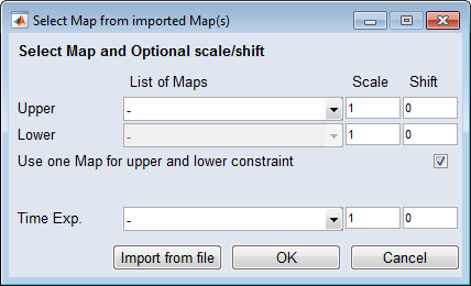
Afterwards, the borders can be slightly extended by adding scales and shifts for the lower and upper limits with Scale/Shift.
For more information about editing map data, see Parameter/Model ® Edit.
|
Note |
|---|
|
To extend the lower borders, the value of the shift must be negative. |
Exporting map data
Map data can also be exported, using the Export button, as *.dcm or *.csv.
See also the tutorial in the Help (Step 2: Constraints).