Elements of the ASCMO-STATIC User Interface

The following figure shows the user interface of ASCMO-STATIC with an opened project. The main working window shows the modeled dependencies of the outputs on the inputs as intersection plots and is also called ISP view.

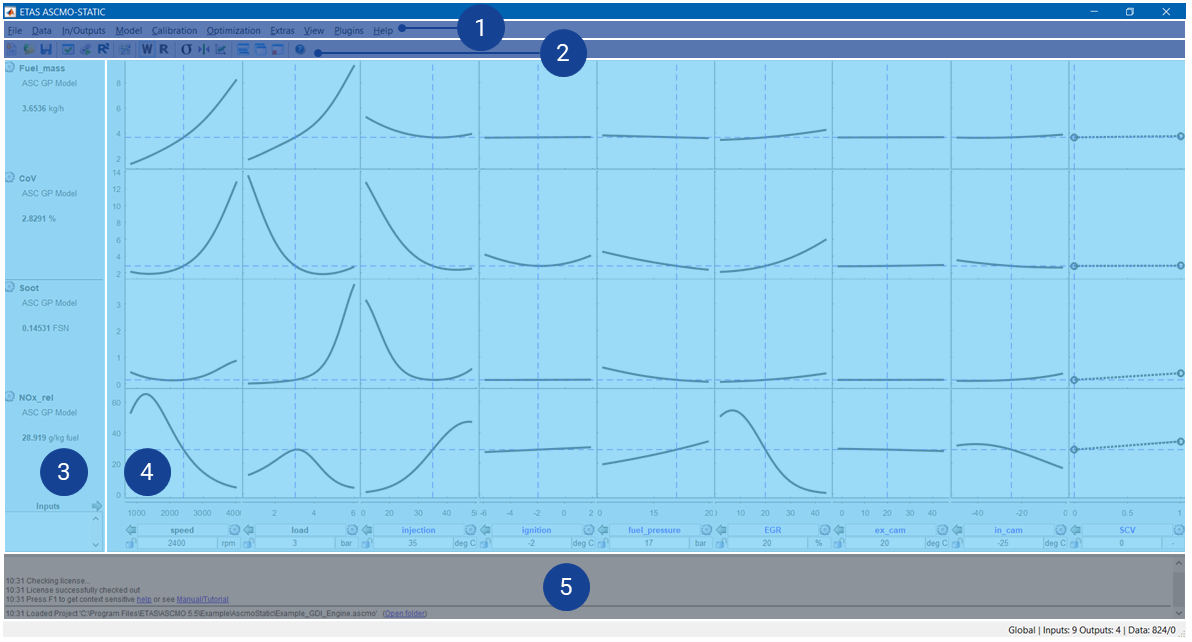
Fig. 55: Graphical user interface (GUI) of ASCMO-STATIC (with opened project)

The GUI is divided into 5 different parts:

• ➀ Main menu
• ➁Toolbar
• ➂Outputs
• ➃ Main working window: Intersection plots (ISP View) and Inputs
• ➄Log window
• Status bar (footer) with current state information

The main menu offers several operations for user activities. In addition, there are a series of interaction possibilities in the areas with the inputs (bottom) and outputs (left) and the intersection plots (see Intersection Plots ) that are described below.

Main Menu

A detailed description of the function of the main menu and the dialog windows associated with it is located in the context-sensitive online help (<F1>).

Inputs

The inputs x1,..., xn (under the intersection plots) and the outputs y1,..., ym (to the left of them) form a matrix at whose intersections the respective intersection plots y1 = f(x1),..., ym= f(xn) are displayed.

In the figure, these are "NOx_rel = f(injection)" and "NOx_rel = f(ignition)".

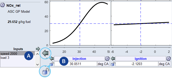
Fig. 56: ISP view: Inputs

• List of hidden inputs (A)

  All inputs not displayed in the ISP view are listed here. Double-click on an entry to show it in the ISP view.

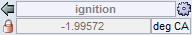
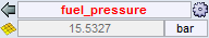
• Name of the respective input (B)

  Clicking on the icon to the right of this field opens the "<input> - Parameters" window.

  

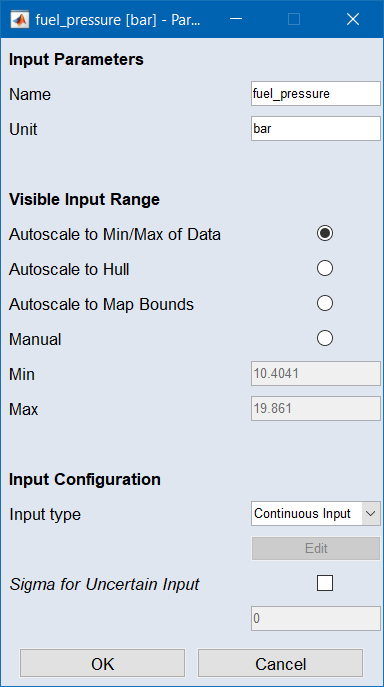
  In that window, you can change input name and unit, set the visible range, and configure the input.

• Current value of the respective input (B)

  A change of the value is made with an entry in this field or by clicking in the intersection plot.

• Hides the corresponding input

  The status (locked/unlocked/use map) is not changed when you remove an input from the display.

• Changes the state of the current input

  The following states are available:

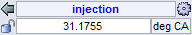
  unlocked	The value can be changed manually and by the optimization. The input name appears in blue, and the value field (2) can be edited.
  locked	The value is fixed. It cannot be changed manually or by the optimization. The input name appears in gray, and the value field (2) is set to read-only.
  use map	The input value is interpolated from the respective calibration map at the point of the current speed and load. The input name appears in red, and the value field (2) is set to read-only.

Outputs

The modeled outputs are displayed to the left of the intersection plots.

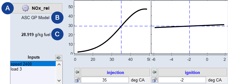
Fig. 57: ISP view: Outputs

• Name of the respective output (A)

  Clicking the button opens the "Output Properties for <output>" window.

  

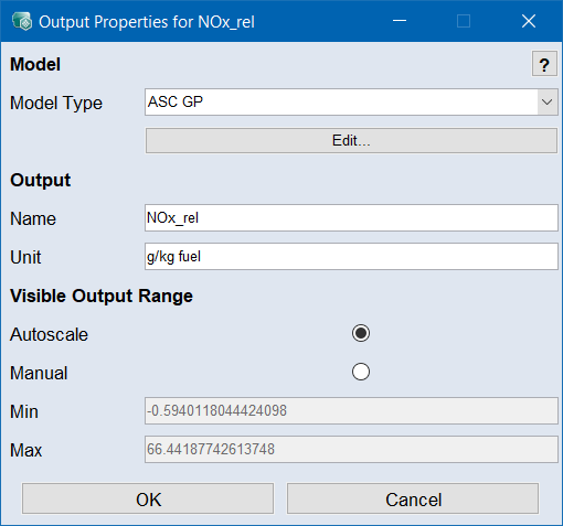
  In that window, you can select the model type, access the model parameters via the Edit button, change output name and unit, and set the visible range.

  For example, the model type can be selected here. The transformation of an output (see Model Improvement Through Transformation of Output Variables) can be manually defined in the model type parameters, accessible via the Edit button. Details about the meaning of the other settings can be found in the online help (<F1>).

• Model type of the output (B)

  Clicking on the model type name opens the model parameter window; see Model Types of ASCMO-STATIC for further information on the model types.

• Current value of the output (C)

  Current value of the output (corresponding to the selected value of the respective input).

Log Window

The bottom part of the main window displays information about executed functions, error messages, etc.

The blue underlined words in the log window are links that give you the ability to access context-sensitive information from the Help system (press F1 to get context-sensitive help in HTML format or see Manual/Tutorial in PDF format) or provide information about activities and functions that can be performed as part of the optimization process (e.g., "Created new project. You should check your training data.")

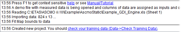
Fig. 58: Information in the log window (example)

 

Save log file

• Right-click in the log window and select Save Log to File from the context menu.

  The "Save Log file As" window opens.

• Specify the file name and click Save.

  The log file is saved.