Intersection Plots

The model training for an output leads to a function of the following form:

youtput = f(xinput_1,...,xinput_n)

With respect to the display, this results in a hyperplane in an n+1-dimensional space that can no longer be graphically displayed as soon as n > 2.

Instead, the main window in ASCMO-STATIC shows n intersections through this hyperplane, the so-called intersection plots. With each of these intersections, only one dimension is being varied, while the values of the other dimensions are kept constant, resulting in

youtput = f(xinput_1), ..., youtput = f(xinput_n)

With n inputs and m outputs, this results in n x m intersection plots. The inputs x1, ..., xn (in the user interface underneath the intersection plots) and the outputs y1, ..., ym (to the left of them) form a matrix at whose intersections the respective intersection plots y1 = f(x1), ..., ym= f(xn) are displayed.

This is shown again in Fig. 62 for the case to be displayed of the dependency of one output on two inputs.

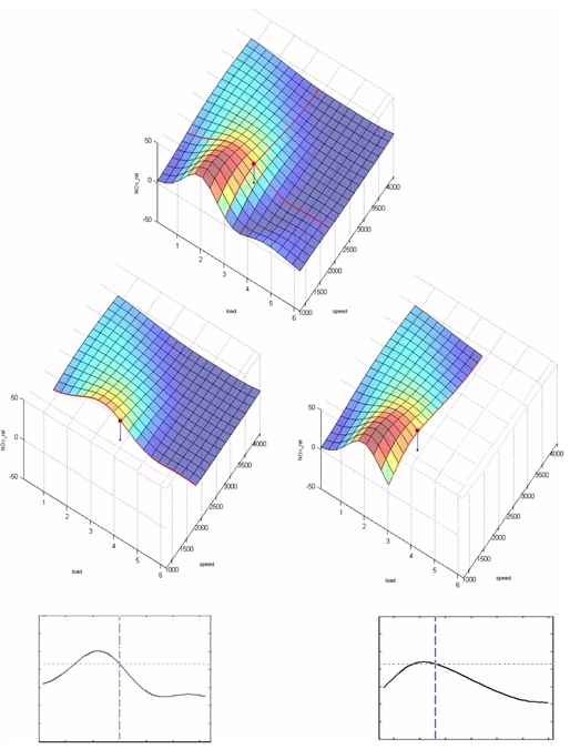
Fig. 62: Intersection plot as 2-dimensional intersections in the n+1-dimensional hyperspace (here: n = 2)

The example in the figure shows the model of the dependency of the output NOx_rel (relative nitrogen oxide emission) on speed and load.

The first intersection occurs with a plane of constant speed – the result is the functional dependency of the nitrogen oxide emission on the load (on the left in the figure). All other input parameters (only speed in the example) remain constant.

The second intersection occurs with a plane of constant load – in this case, the intersection plot shows the dependency of emission on speed (on the right in the figure).