Interactions <output>
Model menu > Interactions ><output>
The degree of interaction of two inputs on the respective output is graphically displayed in this window.
In every individual diagram, an input variable (the column) is continuously being varied, a second input variable (the row) features three discrete values Min, Mean and Max, which results in three graphs per diagram.
A significant interaction between two inputs each is present if the graphs in a diagram do not run parallel or even intersect.
 Example: Interpreting model output plots
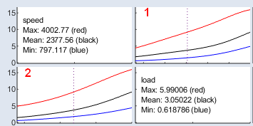
Plot 1 explores how the model output changes with varying load at different fixed speed levels:
-
Red line: Speed = 4002 (maximum of speed). Load varies from 0.6 to 5.99.
-
Black line: Speed = 2377 (mean of speed). Load varies from 0.6 to 5.99.
-
Blue line: Speed = 797 (minimum of speed). Load varies from 0.6 to 5.99.
Plot 2 explores how the model output changes with varying speed at different fixed load levels:
-
Red line: Load = 5.99 (maximum of load). Speed varies from 797 to 4002.
-
Black line: Load = 3.05 (mean of load). Speed varies from 797 to 4002.
-
Blue line: Load = 0.62 (minimum of load). Speed varies from 797 to 4002.
The dotted vertical line marks the setting of all other input variables used in the calculation.
By default, this corresponds to their mean values, but you can adjust them interactively by clicking the plot.
Each figure therefore illustrates the interaction between two inputs, while holding the others constant.
How to read the plots:
-
Flat line: No interaction between the two inputs.
-
Steep upward trend: Positive interaction between the two inputs.
-
Steep downward trend: Negative interaction between the two inputs.
-
Crossing lines: Strong interaction; the output’s increasing or decreasing behavior changes depending on the setting of the other input.
|
Note |
|---|
|
The values of the inputs are displayed by the dashed blue line and can be set here just like in the ISP view. |