Phase Plot, ACF and IACF

Data > Phase Plot and IACF Outputs makes it possible to identify the time dependency of the identification task. Each output is shown in a different window.

Phase Plot

A scatter plot of output(k) over output(k-t); the phase/lag t can be adjusted in the lower left corner of the window (the standard value is 1).

This plot (top half of Phase plot and ACF/IACF plot for an output) shows the changes of the output values over time from one step to the t-th following. Many points on the diagonal with slight scattering indicate a strong dependency between the output(k) and the phase-shifted output(k‑t). This is normally the case for a phase of t = 1. If you increase t in steps, the point distribution approximates equal distribution – this means you can estimate the time dependency of an output.

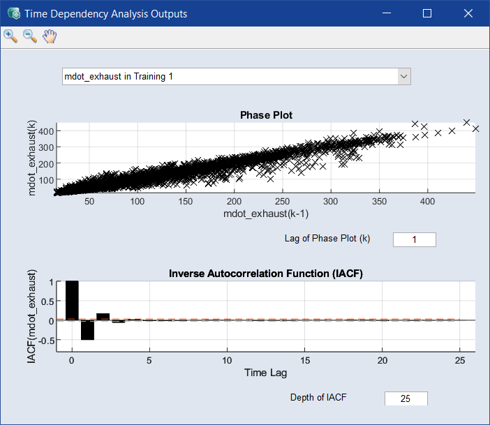
Fig. 35: Phase plot and ACF/IACF plot for an output

Autocorrelation Function (ACF)/Inverse Autocorrelation Function (IACF)

The analysis with ACF and IACF assumes a linear time series with no external input variables involved. Of course, this is not the case in the identification of non-linear systems, e.g. the diesel engine example, but we can draw some first assumptions from this about the present time dependency.

The expected shape of the ACF is exponentially decreasing or sinusoidal. A sudden decay after a few time lags would indicate no autoregressive part (no time dependency) within the time series.

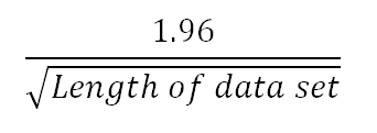
The IACF plot (bottom half of Phase plot and ACF/IACF plot for an output) should decay after a few steps, which gives the order of the autoregressive part. The dashed line represents the cut-off criterion, which is the 95% confidence interval:

Exponential or sinusoidal behavior of the IACF would indicate no autoregression. In the diesel engine example, the IACF decays after a signal shift of 3 time lags. This is the time lag horizon to be considered for the upcoming model training.