Phase Plot and ACF/IACF Outputs

The "Time Dependency Analysis Output" window, opened via Data → Phase Plot and ACF/IACF Outputs in the main window, allows you to identify the time dependency of the identification task.

Phase Plot

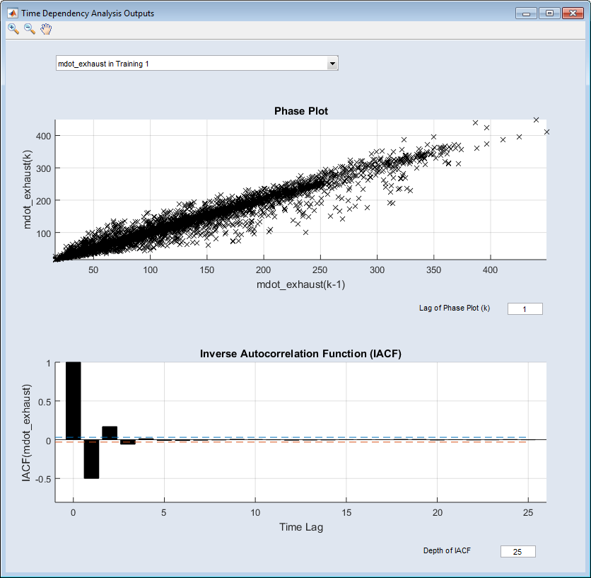
A scatter plot of <output>(k) over <output>(k-t); the phase/lag t can be adjusted in the "Lag of Phase Plot (k)" field below the bottom-right corner of the phase plot; the default value is 1.

This plot shows the changes of the output values over time from one step to the t-th following step. A strong dependency between <output>(k) and the phase-shifted <output>(k-t) is indicated by there being many points on the diagonal. This is normally the case for a phase of t = 1. If you increase t in steps, the point distribution approximates equal distribution – this means you can estimate the time dependency of an output.

Autocorrelation Function (ACF)/Inverse Autocorrelation Function (IACF)

The analysis with ACF and IACF assumes a linear time series with no external input variables involved. Of course, this is not the case in the identification of non-linear systems, but you can draw some first assumptions from this about the present time dependency.

The expected shape of the ACF is exponentially decreasing or sinusoidal. A sudden decay after a few time lags would indicate no autoregressive part (no time dependency) within the time series.

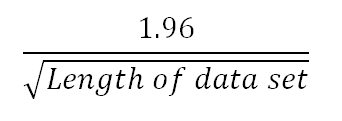
The IACF plot should decay after a few steps, which gives the order of the autoregressive part. The dashed lines represent the cut-off criterion, which is the 95% confidence interval:

Exponential or sinusoidal behavior of the IACF would indicate no autoregression. If for example, the IACF decays after a signal shift of 3 time lags, this is the time lag horizon to be considered for the upcoming model training.