Nonlinear Autoregression With Exogenous Inputs (NARX)

Dynamic effects with a data-driven modeling algorithm, e.g. the ASC modeling part of ASCMO-DYNAMIC, can be taken into consideration by using a superordinate model structure. In the discrete time case, the system input space is expanded with the feedback of past input and output values up to a certain time horizon, as shown in Fig. 67. This is referred to in literature as nonlinear autoregression with exogenous inputs (NARX). The feedback values are referred to as features in the following.

With this approach, the dynamic identification problem is transformed into a quasi-stationary relationship:

y(k)=f(x_1 (k),x_1 (k-1),…,x_2 (k),x_2 (k-1),…,y(k-1) ,…)

where k indicates the discrete time-step.

Based on a continuously measured data set of the system inputs and outputs, the ASC modeling algorithm, or any other data-driven regression, can be applied for the modeling of the functional relationship f( ).

Multi-Step vs. One-Step Ahead Prediction

After model training, we can distinguish between two scenarios for the application of the model in the prediction (see Fig. 67):

• One-step ahead prediction

  In the case of a one step-ahead prediction, the past system outputs are known and given by actual measurements, e.g. through sensors. The model has to predict just the upcoming time step.

• Multi-step ahead prediction

  In the multi-step ahead prediction, the past system output values are replaced by the model’s predictions. This corresponds to an offline simulation and is the standard use case, where the user wants the model response to a given set of input variations.

  Compared to the one-step ahead implementation, the multi-step case usually results in a worse model quality due to the accumulation of prediction errors.

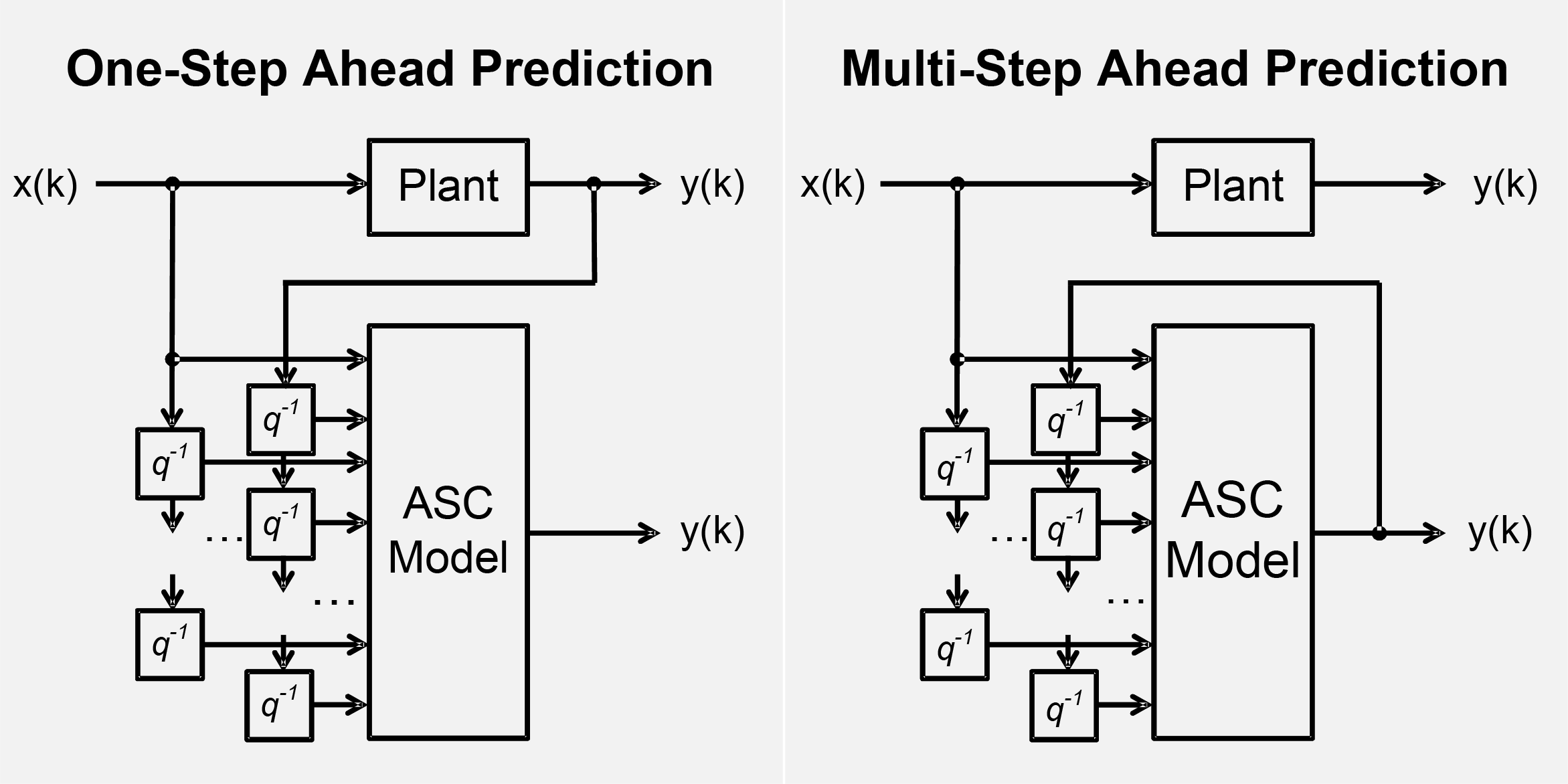
Fig. 67: Model structure for nonlinear autoregression with exogenous inputs (NARX)

See also section Multi-Step/One-Step Ahead Prediction .