Multi Result Optimization

Optimization menu > Multi Result

Performs a multi-criterial local optimization at the selected operating point.

Multi result optimization enables a true multi-goal optimization, i.e. there is no weighting of output variables.

In the Multi Result Optimization window, the necessary criteria and values can be set.

The Multi Result Optimization window contains the following elements:

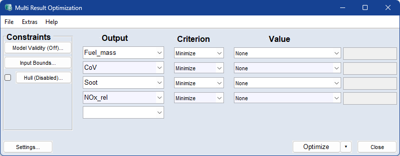
Closed File

Closed Extras

Closed Help

Constraints

Model Validity

Opens the Valid Model Range window. In that window, you can restrict optimization of each criterion to the respective valid model range.

Note
The valid mode range makes the optimization slow and no solution might be found at all, because the valid regions are not contiguous. In many cases it is better to constrain the solutions to the Input Bounds > Fit all Bounds to Data, see next constraint option.

Note

The valid mode range makes the optimization slow and no solution might be found at all, because the valid regions are not contiguous.

In many cases it is better to constrain the solutions to the Input Bounds > Fit all Bounds to Data, see next constraint option.

Input Bounds

Opens the Input Bounds window where you can define the range to be considered for the modeling for each input.

Checkbox and Hull (*)

If the checkbox is enabled, the button is named Hull (2D). Otherwise, the button is named Hull (Disabled).

The button opens the Configure Convex Hull on Inputs window where you can configure 2D, 3D, and/or 4D hulls.

Note
You must activate the checkbox manually even if you clicked Hull (Disabled) and configured hulls.

Output

The drop-down lists in this column offer all outputs for selection. In addition, the Remove entry can be used to delete a row.

Criterion

Here, you select the optimizing criterion for the respective output. Available selections are:

Minimize/Maximize

The optimizing goal consists of minimizing/maximizing the output.

In addition, a hard upper and/or lower limit can be defined in the Value column.

Target

A target value which should be reached as closely as possible.

In the Value column, the value can be set as global (Constant) or per OP.

Bound

(Upper or lower) limit value for the optimizing goal.

In the first Value column, the limit can be further specified.

See also Optimization Criteria.

Value

In the Value columns, you can fine-tune the criterion.

criterion	possible selections in 1st "Value" column	input in 2nd "Value" column
Minimize, Maximize	None	(column is empty and disabled)
	Hard Lower Bound	value of lower/upper bound
	Hard Upper Bound	value of lower/upper bound
	Hard Lower&Upper Bounds	values of lower and upper bounds (the column is split in two)
Target	Target	target value
Bound	Hard Upper Bound	value of lower/upper bound
	Hard Lower Bound
	Weak Upper Bound
	Weak Lower Bound
	Hard Lower&Upper Bounds	values of lower and upper bounds (the column is split in two)

Settings

Opens the Settings window for multi result optimization.

Optimize

Performs the optimization starting at the current position in the ISP. Operating Point Axes should be locked in the ISP, to find an optimization for a specific Operating Point.

Results are displayed in the log window, and calculated values appear in the ISP view. A window opens in which the outputs to be represented can be selected (see The Plot of n Pareto Optimal Solutions Windows). The results are several pareto-optimal solutions, i.e. different combinations of all setting parameters for the different optima.

Use for further options:

Export Job to Docker: Exports the single result optimization information as *.docker.ascmo file. Use the file to perform the optimization in a Docker container, e.g., in the cloud.

Closes the window without staring an optimization. Changed setting are kept.