Algorithmic Details of Symbolic Regression
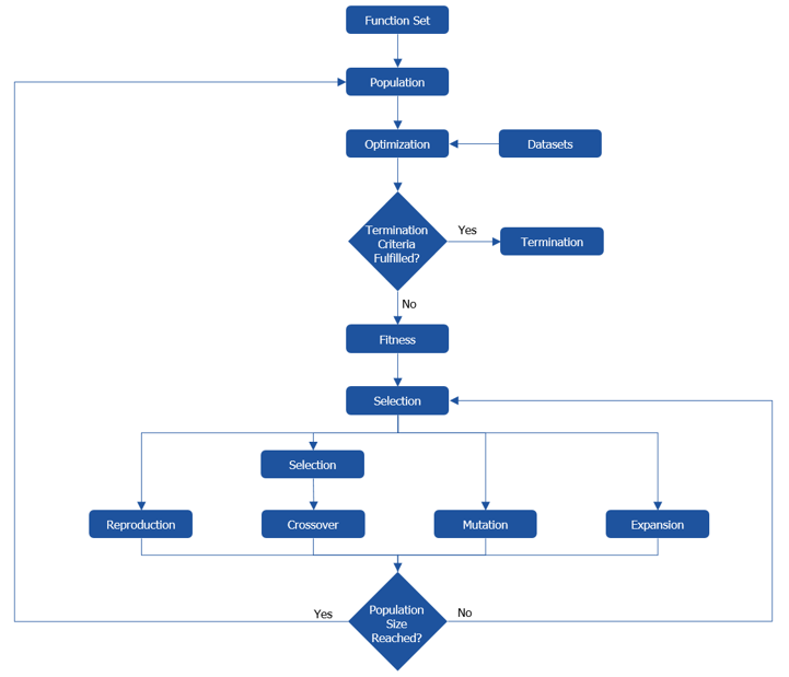
To carry out symbolic regression, ASCMO-MOCA uses a modified version of genetic programming. The algorithm is specifically suited to fulfill the required task. The major algorithmic steps are described below and in the image.
A set of functional expressions is defined which are used during the course of the algorithm. In ASCMO-MOCA this step is covered by choosing the function/operation types you want to use by clicking on the elements in the "Selected Alphabet" area.
After the function set is defined, a population/set of models is created on a stochastic basis. Starting with this step the models are represented as graphs. The creation process is constrained w.r.t. the population size and the graphs' dimensions. During the course of the algorithm the population evolves from the evolution operations. Each iteration-step in the main loop of the algorithm corresponds to one generation.
|
Note |
|---|
|
See also each field tooltip for more information. You can also open them in an extra window by clicking on it. |
Corresponding Configuration Parameters (Optimization Configuration & Initial Configuration) in the "Symbolic Regression" window
- Random Seed: Integer used as the seed for the random number generation, which effects all stochastic steps within the algorithm. Modify this value to improve the performance in critical cases.
- Population Size: Number of models contained in each population. For hard problems population sizes of several thousands have performed well.
- Population Creation Method (Initial Configuration): The initial population is created with one of the three different methods. For unknown problems the half-and-half methods is a good choice.
- half and half: One half of the population is created with full method and the other half of the population is created with the grow method. The used maximum depth value is determined from a uniform distribution within Population Init Depth Min and Population Init Depth Max, for each graph individually.
- full: Each graph is created such that it has a depth of Population Init Depth Max in all branches.
- grow: Each graph is created such that at least one branch has a depth of Population Init Depth Max.
- Population Init Depth Min: Minimum initial depth.
- Population Init Depth Max: Maximum initial depth. Graphs with a depth of ten are already huge and very complex. Numbers around four are more appropriate.
- Max Program Complexity (Optimization Configuration): No graphs are created (initially and during evolution) having a larger complexity. A graphs' complexity is an integer given by the sum of complexities of all nodes the graph is made of. Node complexities are defined ASCMO-MOCA internally based on experience. Using this option offers you to fasten the algorithm's execution if you have a clear expectation and experience on the complexity for your symbolic regression problem.
-
Max Program Depth: No graphs are created (initially and during evolution) having a larger depth.
-
Max Program Size: No graphs are created (initially and during evolution) having a larger size (number of nodes).
Naturally, symbolic regression requires one or several datasets to be carried out.
For each graph an individual and local optimization is performed. The goal of this optimization is to minimize the value obtained by using the method given by the Fitness Method.
Corresponding Configuration Parameters (Optimization Configuration)
- Optimizer Method
- Levenberg-Marquardt method (LM)
- Trust-region-reflective method
- Dogbox algorithm
- Optimizer Iterations: Maximum number of iterations the local optimization should be carried out.
The algorithm stops if one of the following criteria holds:
- It holds for one of the models in the population that the value obtained by using the method given by the Fitness Method is smaller than the termination threshold.
- The maximum number of generations is reached.
Corresponding Configuration Parameters (Optimization Configuration)
- Termination Threshold: Threshold used for termination. The threshold is a positive double.
- Number of Generations: Maximum number of generations.
For each model in the population it's fitness is computed. To do so the raw-fitness is computed as the sum of two parts:
- The value obtained by using the method given by the fitness method, the cost-function.
- A scalar value penalizing the complexity of the graph.
The actual fitness itself is obtained from normalizing the raw-fitness to values within [0,1].
Corresponding Configuration Parameters (Optimization Configuration)
- Fitness Method: Various cost-function types are available.
- rmse Root mean squared error.
- mse Mean squared error.
- abs Normalized absolute difference (mean of L^1-norm).
- Parsimony Coefficient: Factor to weight the impact of the complexity penalty. For unknown problems, a value of 1 is a reasonable starting point. For smaller values of the Parsimony Coefficient the formula gets more complex.
The structural optimization of the graphs starts with selecting graphs from the population. The selection is done on the basis of the fitness obtained in the previous step, with the methods described below.
Corresponding Configuration Parameters (Optimization Configuration)
- Program Selection Method:
- tournament: From the given population Tournament Size graphs are randomly drawn from the population and the one with the best fitness is selected.
> Tournament Size: Number of programs to select from tournament. Choosing the minimum of 2 individuals will lead to highly volatile progress of the algorithm. If the number converges to Population Size, a dominance of the fittest programs is enforced. Choosing about 10% of the Population Size is a good starting point. - fitness-based: A probability distribution is derived from the fitness of all graphs in the current population. This distribution is sampled to select graphs. The fitter a graph is, the more likely it will be selected.
- greedy overselection:The population is divided into a high-fitness group and a low-fitness group. For both groups fitness-based selection is used. If the high-fitness group is used it is determined with Probability Top. Otherwise the low-fitness group is chosen.
> Fraction Top: The fraction of the population defines the size of the high-fitness group. The group is filled with the graphs having the highest fitness.
> Probability Top: Probability with which the high-fitness group is used for fitness-based selection. - multi tournament: Similar to tournament. With a selectable probability, however, fitness/complexity is taken as a criterion instead of just fitness. This option states the a multi-criterial optimization possibilities, only given for a gradient-free technique like genetic programming.
> Tournament Size: Number of programs to select from tournament. Choosing the minimum of 2 individuals will lead to highly volatile progress of the algorithm. If the number converges to Population Size, a dominance of the fittest programs is enforced. Choosing about 10% of the Population Size is a good starting point.
> Probability Fitness: Probability to use fitness/complexity instead of fitness.
- tournament: From the given population Tournament Size graphs are randomly drawn from the population and the one with the best fitness is selected.
The evolution step comprises the graph-modification operations of reproduction, expansion, mutation, and crossover. It is the actual structural optimization step and relies on the graph selected in the previous step. The probabilities for the different techniques determine how likely they are to be applied to this graph.
Corresponding Configuration Parameters (Evolution Probabilities)
For the four options, each probability defines how likely the according option is carried out. The sum of the probabilities has to equal 100.
- Crossover Probability: Setting it in the range of 80 - 90 is a meaningful choice.
- Reproduction Probability: This operation ensures that graphs with a good fitness are likely to be taken-over unchanged to the next generation.
- Expansion Probability
- Mutation Probability
Reproduction
Reproduction of a graph simply means to take it over as-is in the population of the next generation.
Expansion
The expansion of a graph is carried out by:
- randomly selection a terminal node of the graph,
- creating a new random graph with depth two,
- replacing the terminal node by the new graph.
If the expanded graph has a better fitness than the original one, it is taken over to the next generation. Else, the original graph is taken over as-is.
Mutation
A mutation of a graph is be carried out with three different operations, each of them being applied to a randomly selected node of the graph.
- New Tree: The selected node and all sub-nodes are replaced by a newly created graph with a maximum depth of three.
- Hoist: The selected node of the graph is removed, keeping the consistency of the graph. This method helps to prevent bloat of the graphs.
- Point: The selected node is replaced by a random node with the same number of inputs.
How likely which method is applied is determined by the individual probability. The sum of all three probabilities has to equal 100.
Corresponding Configuration Parameters (Mutuation Probabilities)
- New Tree: Probability to carry out the new tree operation.
- Hoist: Probability to carry out the hoist mutation operation.
- Point: Probability to carry out the point mutation operation.
Crossover
The crossover operation essentially is about recombining two graphs to find an even more fitter one. The operation is carried out by the following steps:
-
The graph selected in the previous step is defined as the target graph.
-
A second graph is selected – exactly as described in Program Selection – and defined to be the source graph.
-
In both graphs one node with all its sub-nodes is selected randomly as branches to-be-exchanged.
-
The branch in the target graph is replaced by the branch of the source graph.
The resulting graph is taken over to the population of the next generation.
The evolution operations are applied until the population of the next generation has Population Size number of members.